For each entry, a link to the chapter in which the word first appears is provided.
A
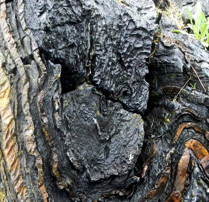
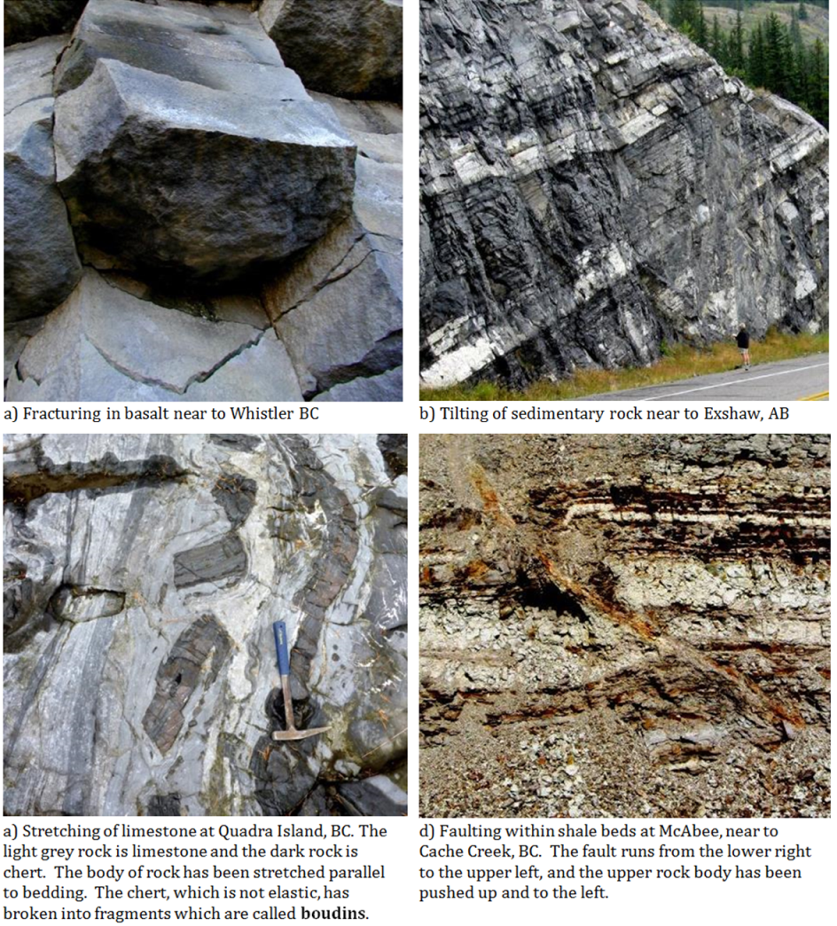
aa (Chapter 4) a lava flow that solidifies with a blocky high-relief surface
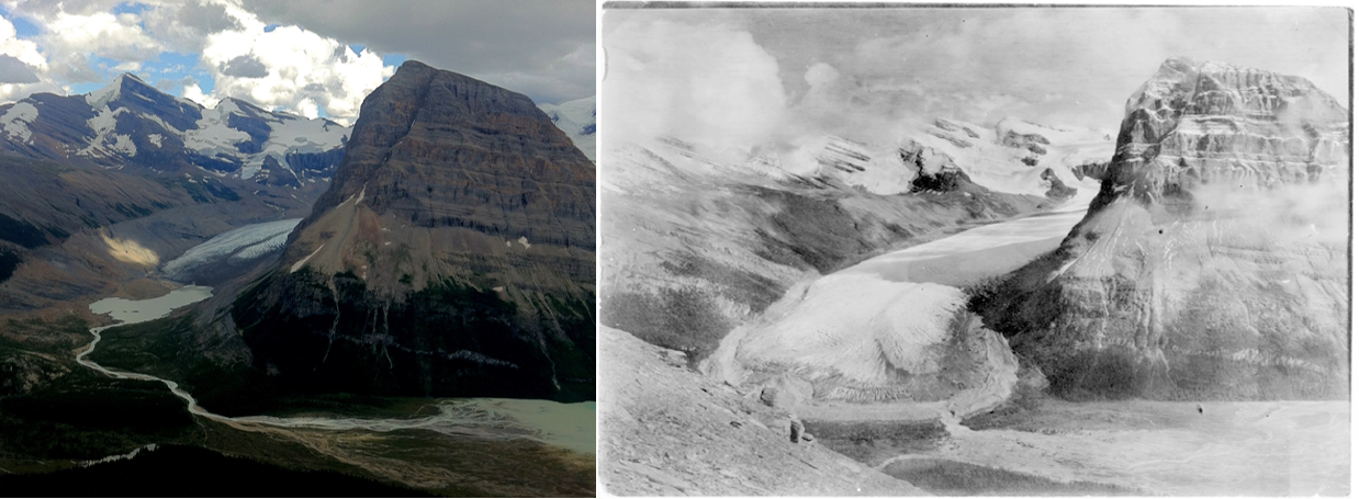
ablation (Chapter 16) melting of ice in the context of glaciation
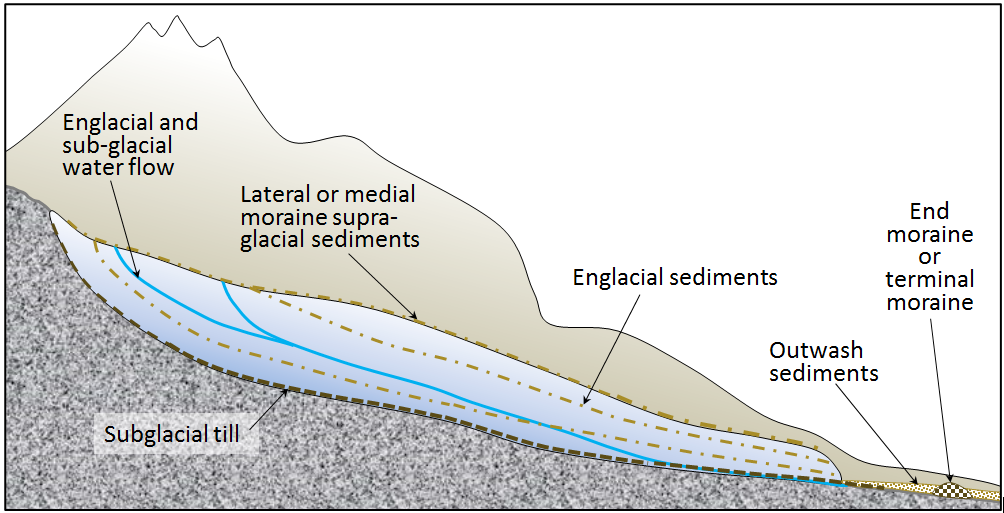
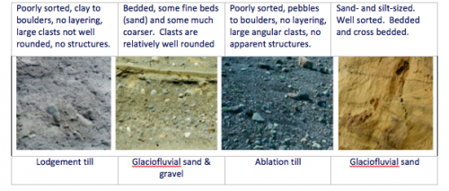
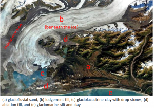
ablation till (Chapter 16) till that is formed when englacial and supraglacial sediments are deposited because the ice that was supporting them melts
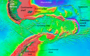
abyssal plain (Chapter 18) the flat surface of the deep ocean, typically beyond the limits of the continental slopes
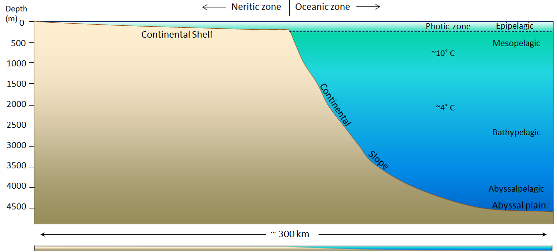
abyssalpelagic zone (Chapter 18) the deeper parts of the ocean, between 4000 and 6000 metres.
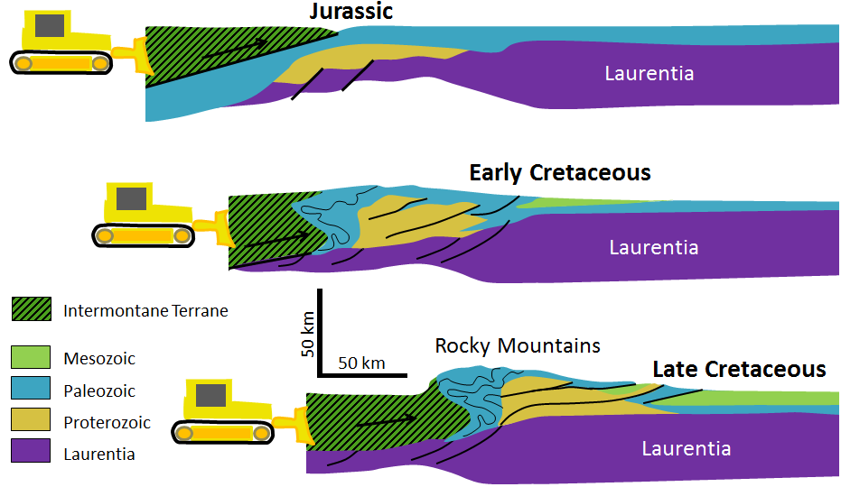
accretion (plate tectonics) (Chapter 21) the process by which continental blocks (terranes) are added to existing continental areas
accretion (planetary) (Chapter 22) the process by which solid celestial bodies are added to existing bodies during collisions
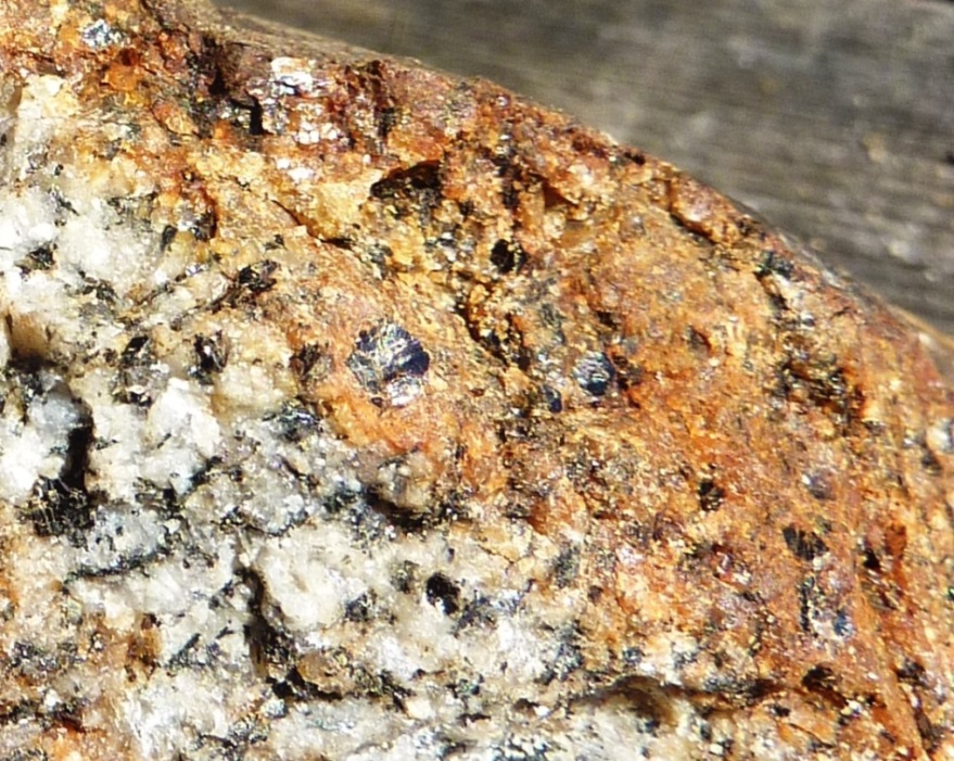
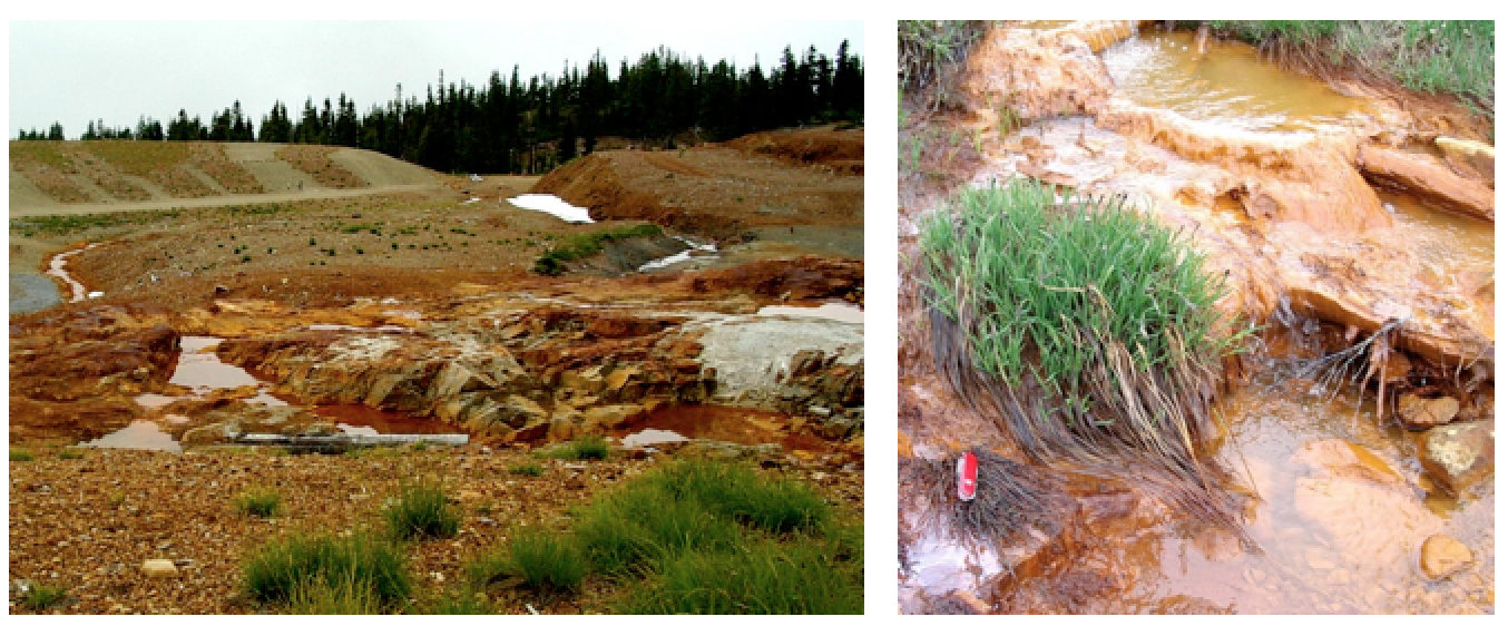
acid rock drainage (Chapter 5) the production of acid from oxidation of sulphide minerals (especially pyrite) in either naturally or anthropogenically exposed rock
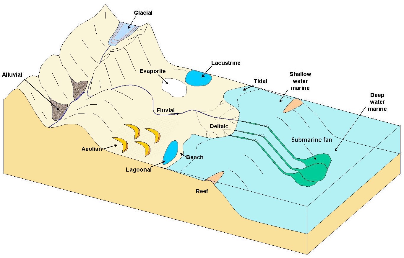
aeolian (Chapter 6) processes related to transportation and deposition of sediments by wind
aerobic (Chapter 18) processes that take place in the presence of abundant oxygen
aerosol (Chapter 4) an aggregate of fine solid particles or a small droplet of liquid suspended in the air
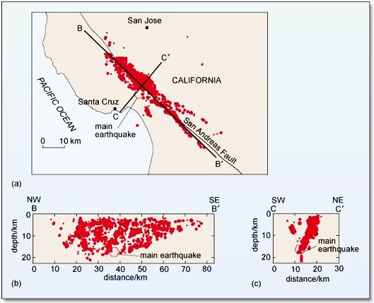
aftershock (Chapter 11) an earthquake that can be shown to have been caused by another earthquake
aggregate (Chapter 20) unconsolidated materials (typically sediments) that are used in the construction industry
albedo (Chapter 19) the reflectivity of a surface of a planet (expressed as the percentage of light that reflects)
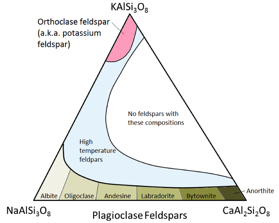
albite (Chapter 2) sodium-rich plagioclase feldspar
alpine glacier (Chapter 16) a glacier formed in a mountainous region and confined to a valley (same as valley glacier)
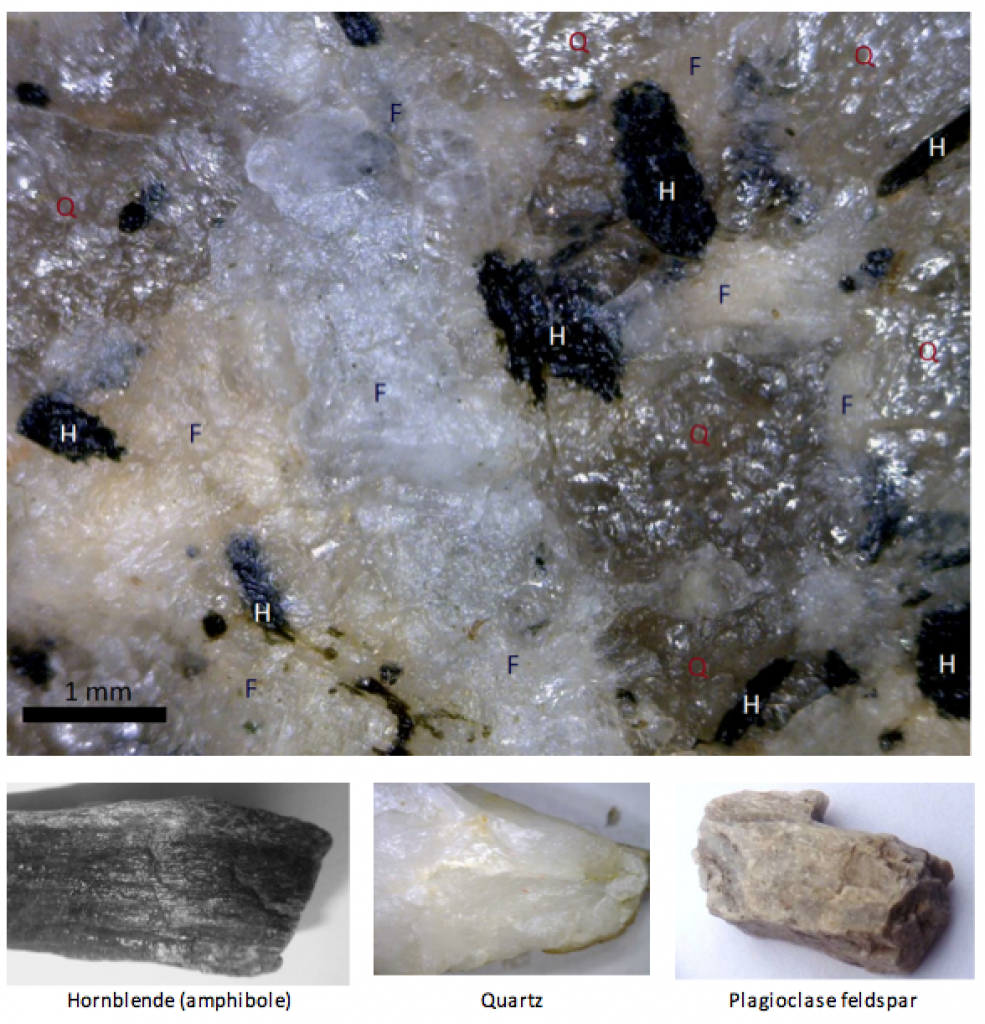
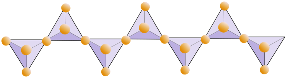
amphibole (Chapter 2) a double-chain ferromagnesian silicate mineral (e.g., hornblende)
amphibolite (Chapter 7) a foliated metamorphic rock in which the mineral amphibole is an important component
amplification (Chapter 11) in the context of seismic shaking the process by which the amplitude of the seismic waves are enhanced, especially because the
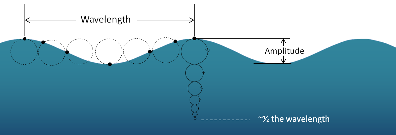
amplitude (Chapter 17) for any type of wave, the difference in height between a crest and the adjacent trough
anaerobic (Chapter 18) processes that take place without oxygen
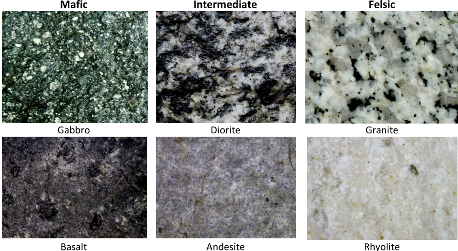
andesite (Chapter 3) a volcanic rock of intermediate composition
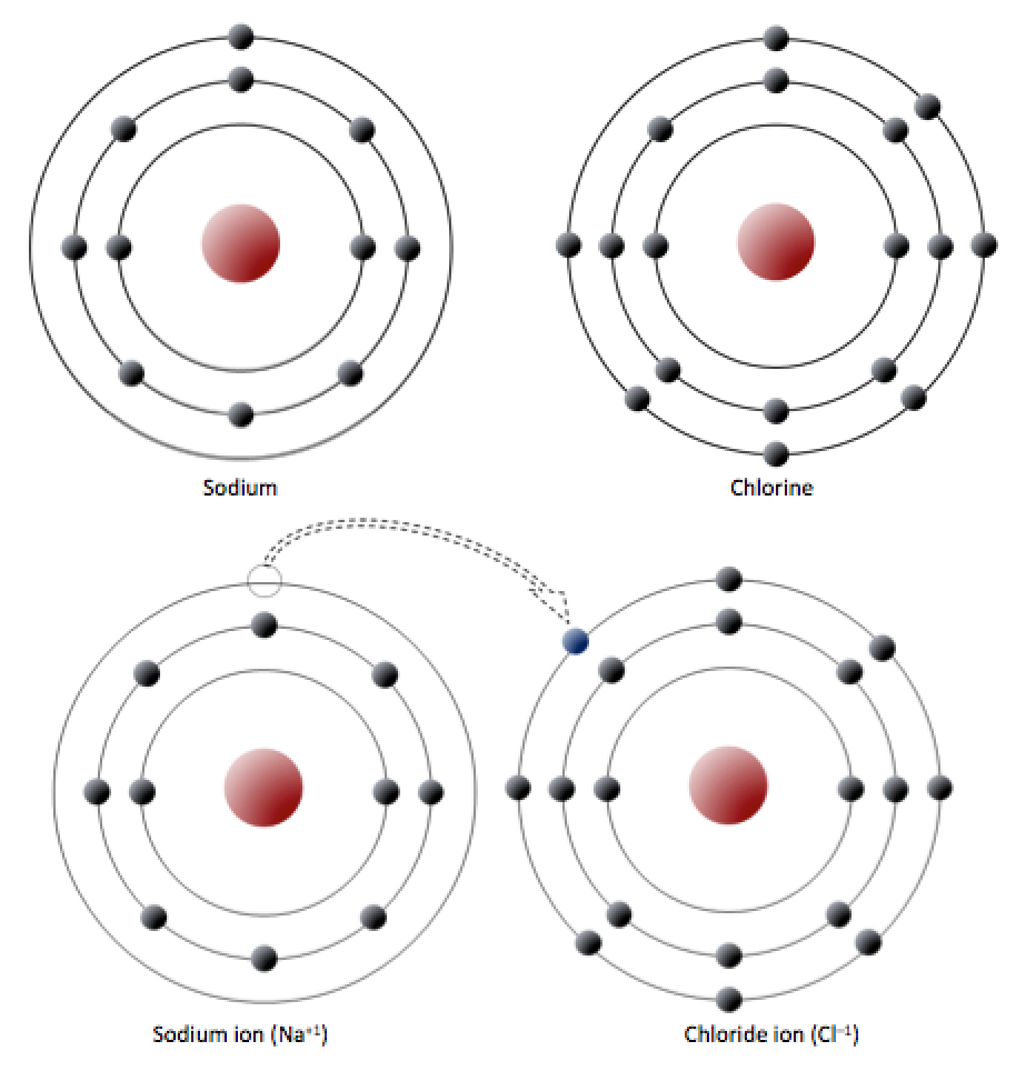
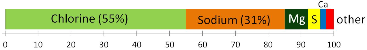
anion (Chapter 2) a negatively charged ion
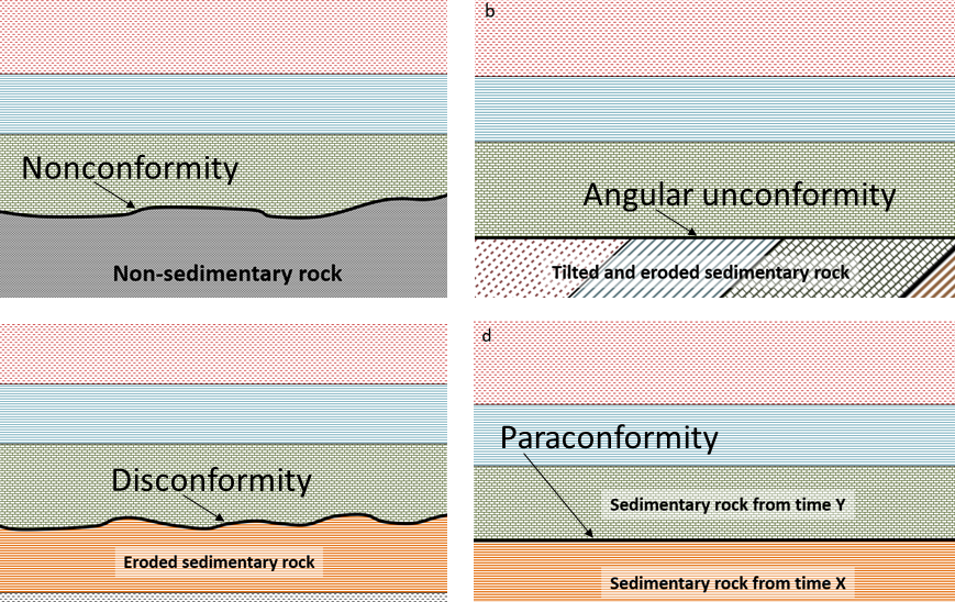
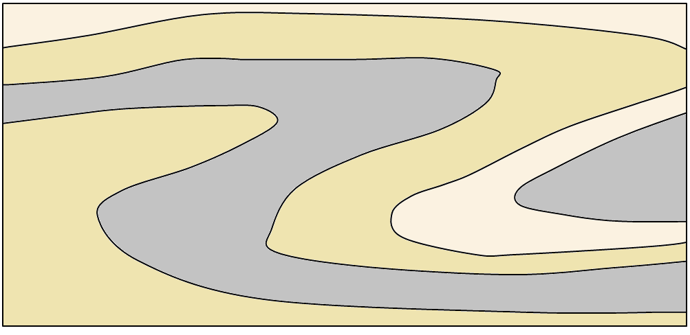
angular unconformity (Chapter 8) a geological boundary at the base of a sedimentary layer where the sedimentary rock beneath has been tilted or folded and then eroded
anorthite (Chapter 2) calcium-rich plagioclase feldspar
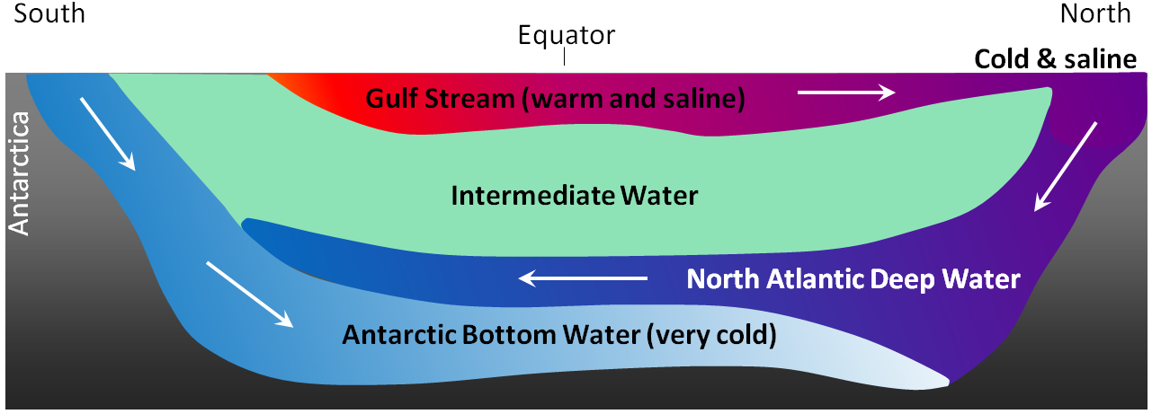
Antarctic Bottom Water (Chapter 18) water at abyssal depths in the ocean that forms from the sinking of dense cold water adjacent to Antarctica
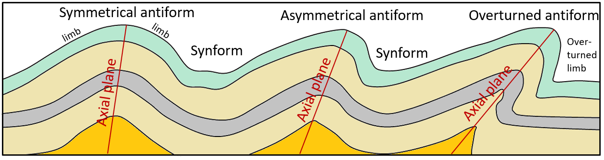
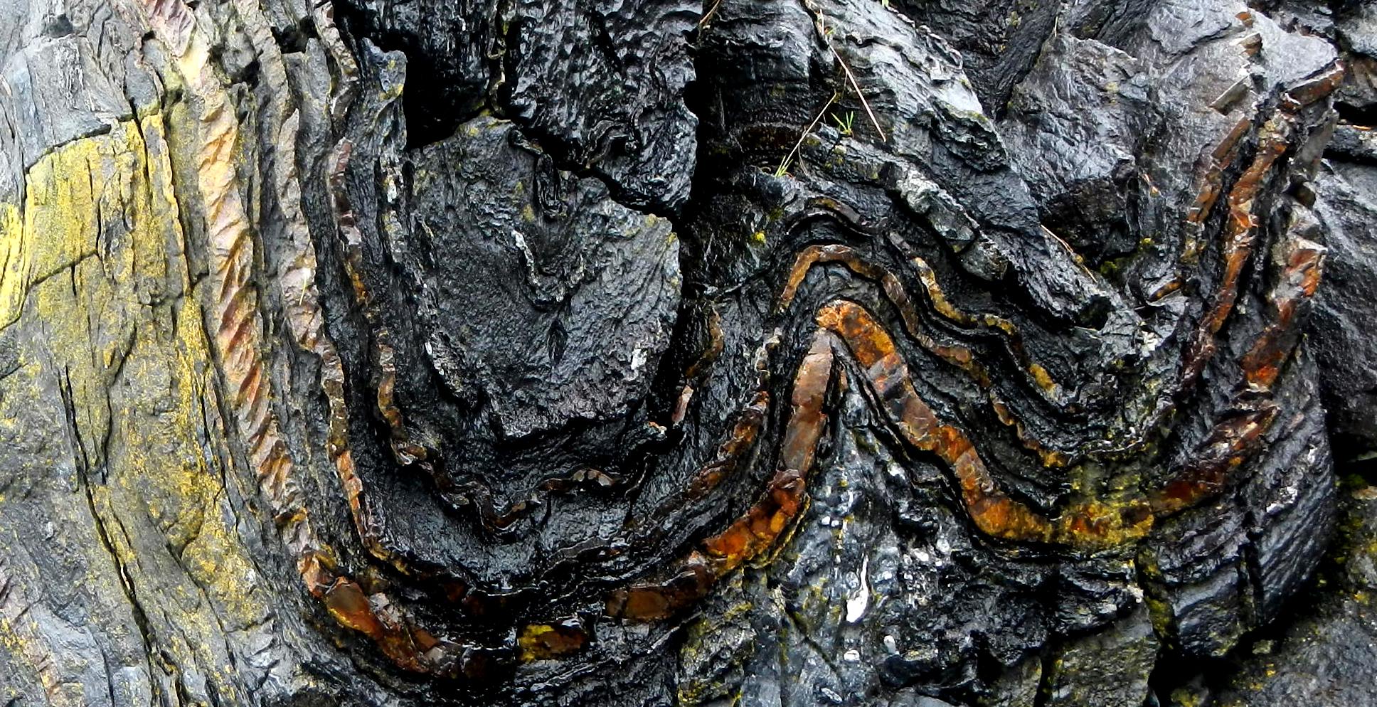
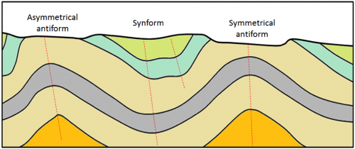
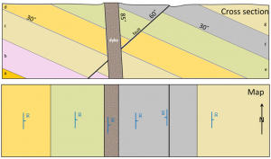
anticline (Chapter 12) an upward fold where the beds are known not to be overturned
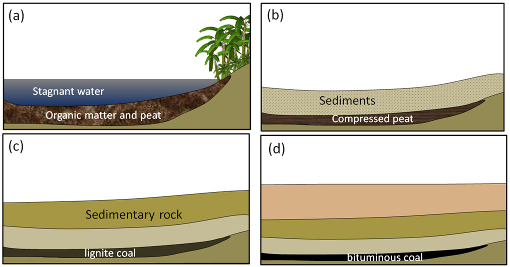
anthracite (Chapter 20) a high grade of coal (92 to 98% carbon) that is formed from deep burial and weak metamorphism
anthropogenic (Chapter 19) resulting from the influence of humans
antiform (Chapter 12) an upward fold where it is not known if the beds have been overturned
aphanitic (Chapter 3) an igneous texture characterized by crystals that are too small to see with the naked eye
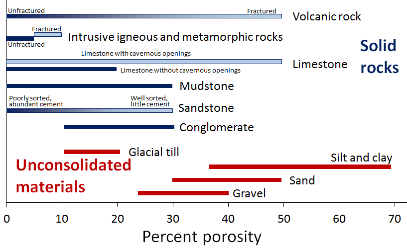
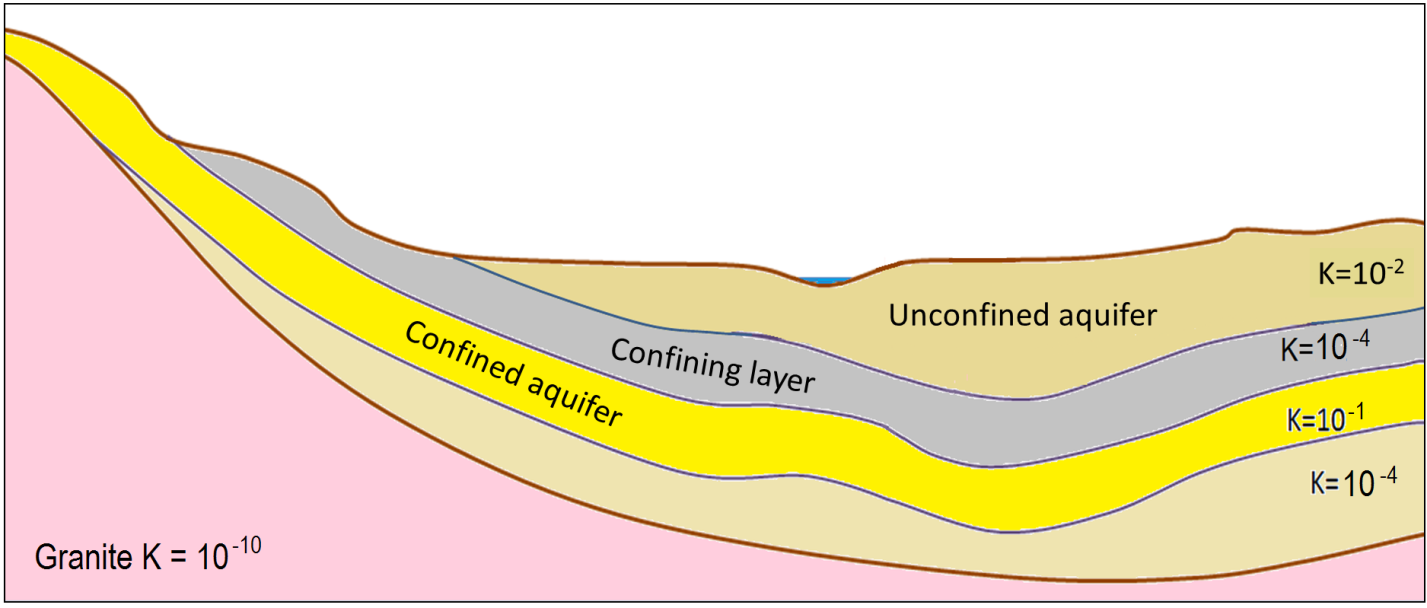
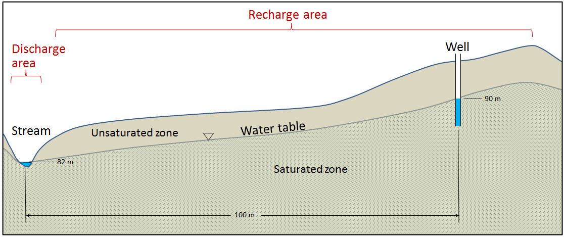
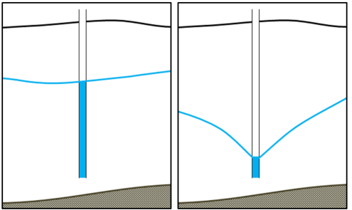
aquifer (Chapter 14) a body of rock or sediment that has sufficient permeability to allow it to be used as a source of groundwater
aquitard (Chapter 14) a body of rock or sediment that has insufficient permeability to allow it to be used as a source of groundwater
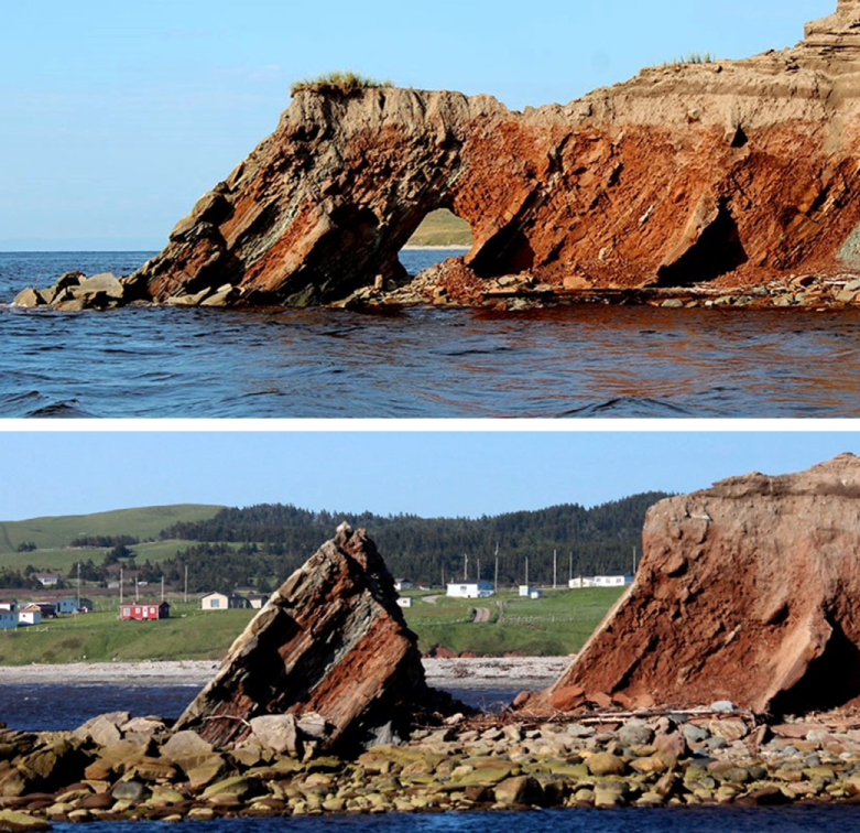
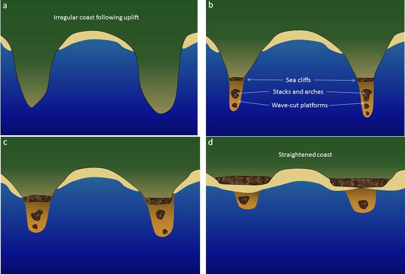
arch (Chapter 17) a rock weathering remnant in the form of an arch (typically along a coast and resulting from wave erosion)
arenite (Chapter 6) a sandstone with less than 15% silt and clay
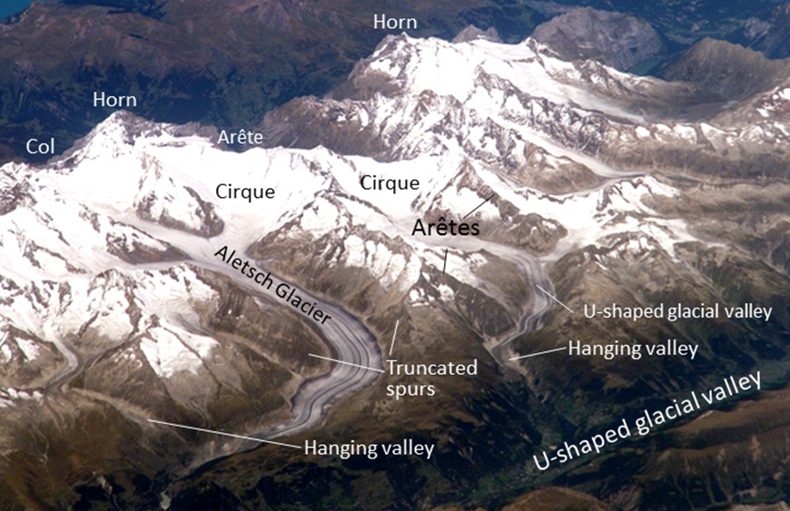
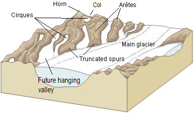
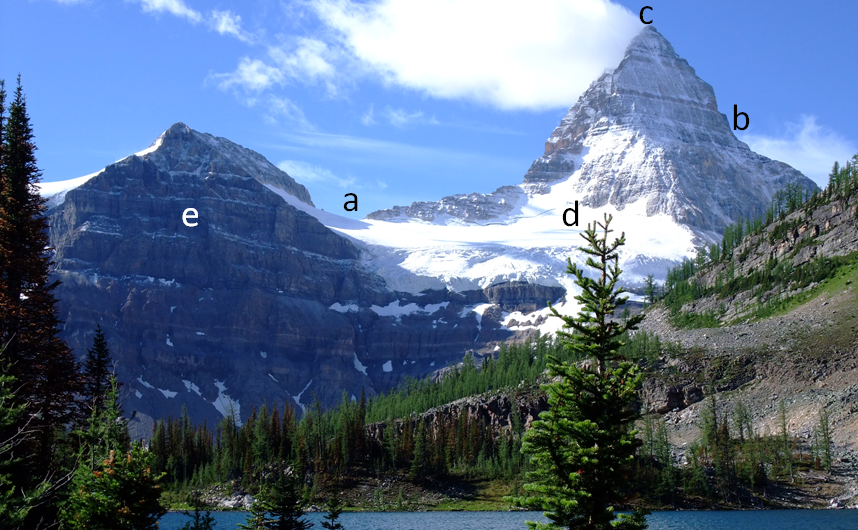
arete (Chapter 16) a sharp ridge that separates adjacent glacially carved valleys
arkose (Chapter 6) a sandstone with more than 10% feldspar and more feldspar than lithic fragments
arkosic arenite (Chapter 6) an arkose with less than 15% clay/silt matrix
artesian well (Chapter 14) a well that is completed in a confined aquifer and in which the water level in the well rises above the top of the aquifer
asteroid (Chapter 22) a rocky body orbiting the Sun
asteroid belt (Chapter 22) the region between the orbits of Mars and Jupiter that is populated with many asteroids
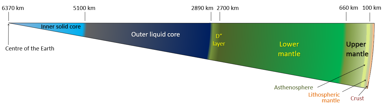
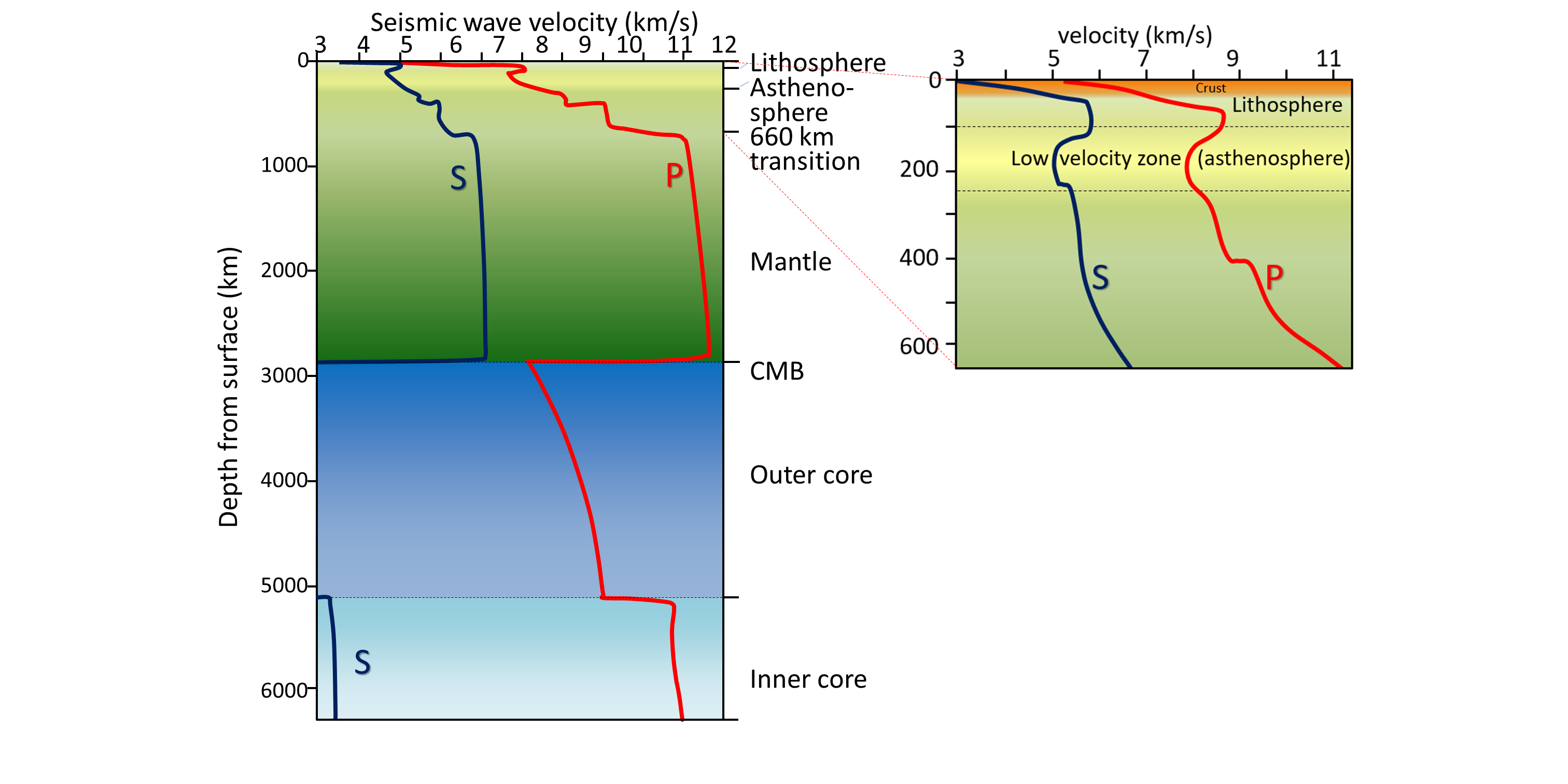
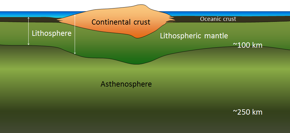
asthenosphere (Chapter 1) the part of the mantle, from about 100 to 200 kilometres below surface, within which the mantle material is close to its melting point, and therefore relatively weak
asymmetrical (Chapter 12) in the context of folds, where the two sides of the fold make significantly different angles with respect to the axial plane
atoll (Chapter 18) a ring-shaped carbonate (or coral) reef or series of islands
atomic mass (Chapter 2) the total number of neutrons plus protons in an atom
atomic number (Chapter 2) the total number of protons in an atom
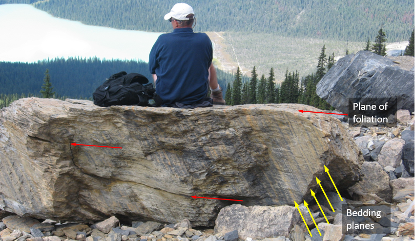
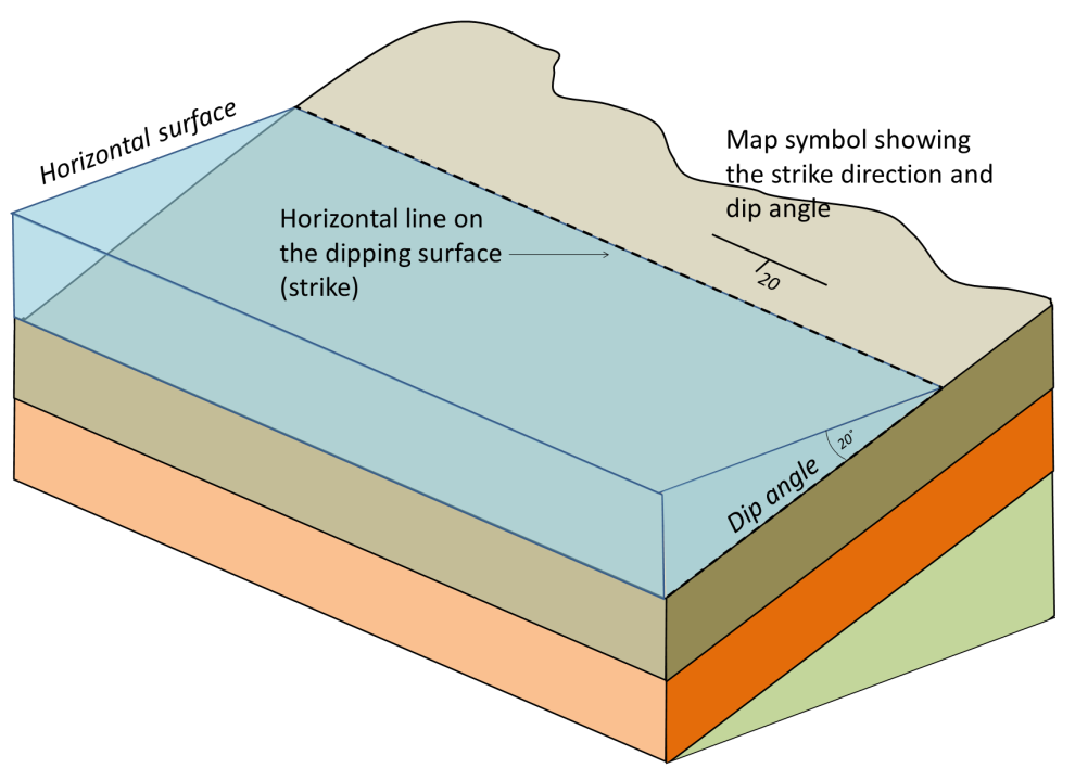
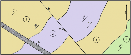
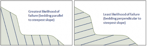
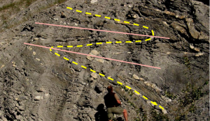
attitude (Chapter 12) the orientation of a sloping geological feature, such as a bedding plane or fracture
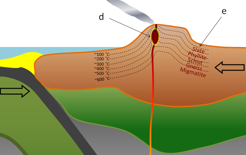
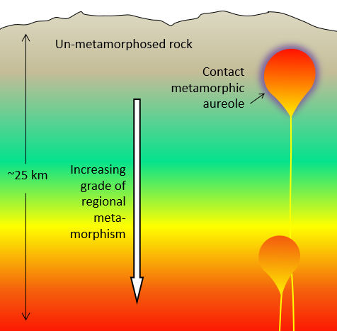
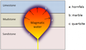
aureole (Chapter 7) a zone of metamorphism around a source of heat such as a magma body
axial plane (Chapter 12) a plane that can be traced through all of the hinge lines of a fold
B
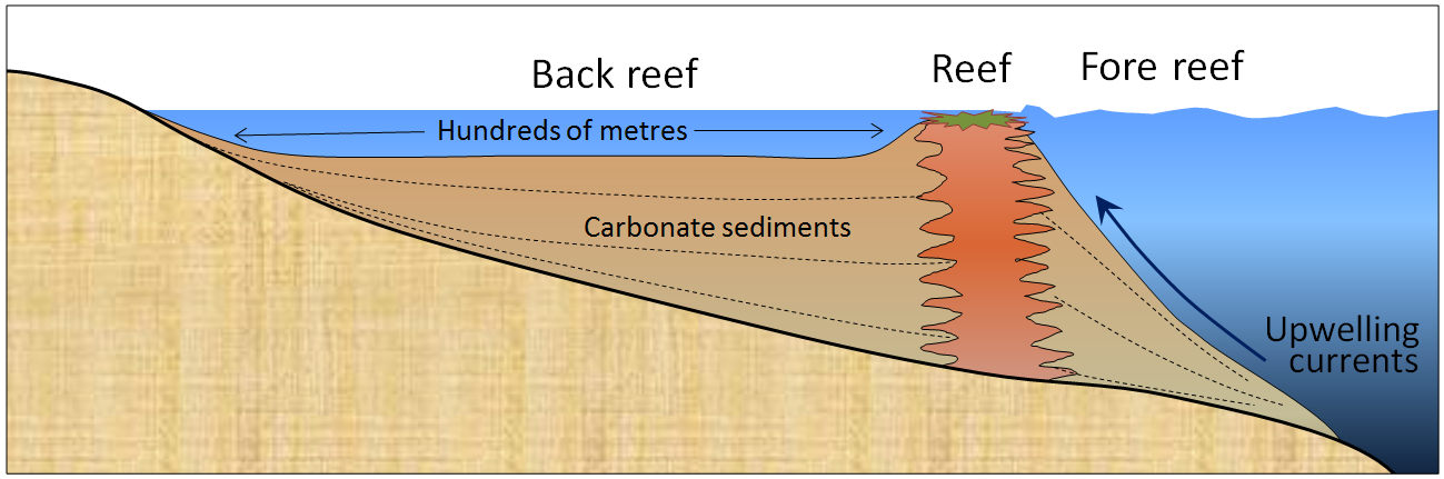
back reef (Chapter 6) the zone of shallow water on the shore-side of a reef
background (geochemistry) (Chapter 20) the typical level of an element in average rocks or sediments
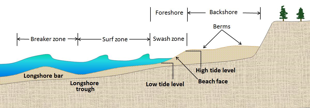
backwash (Chapter 17) the wash of wave water down the slope of a beach
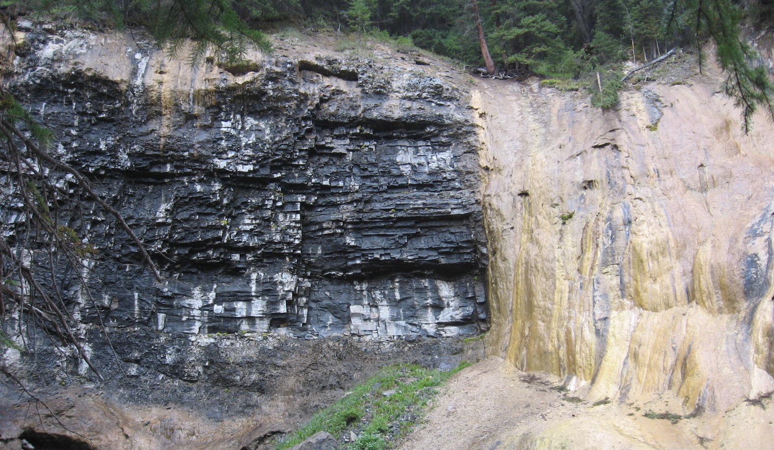
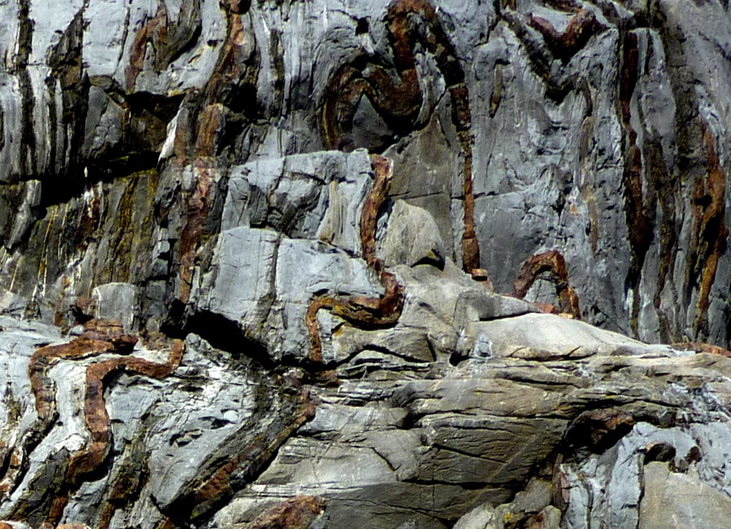
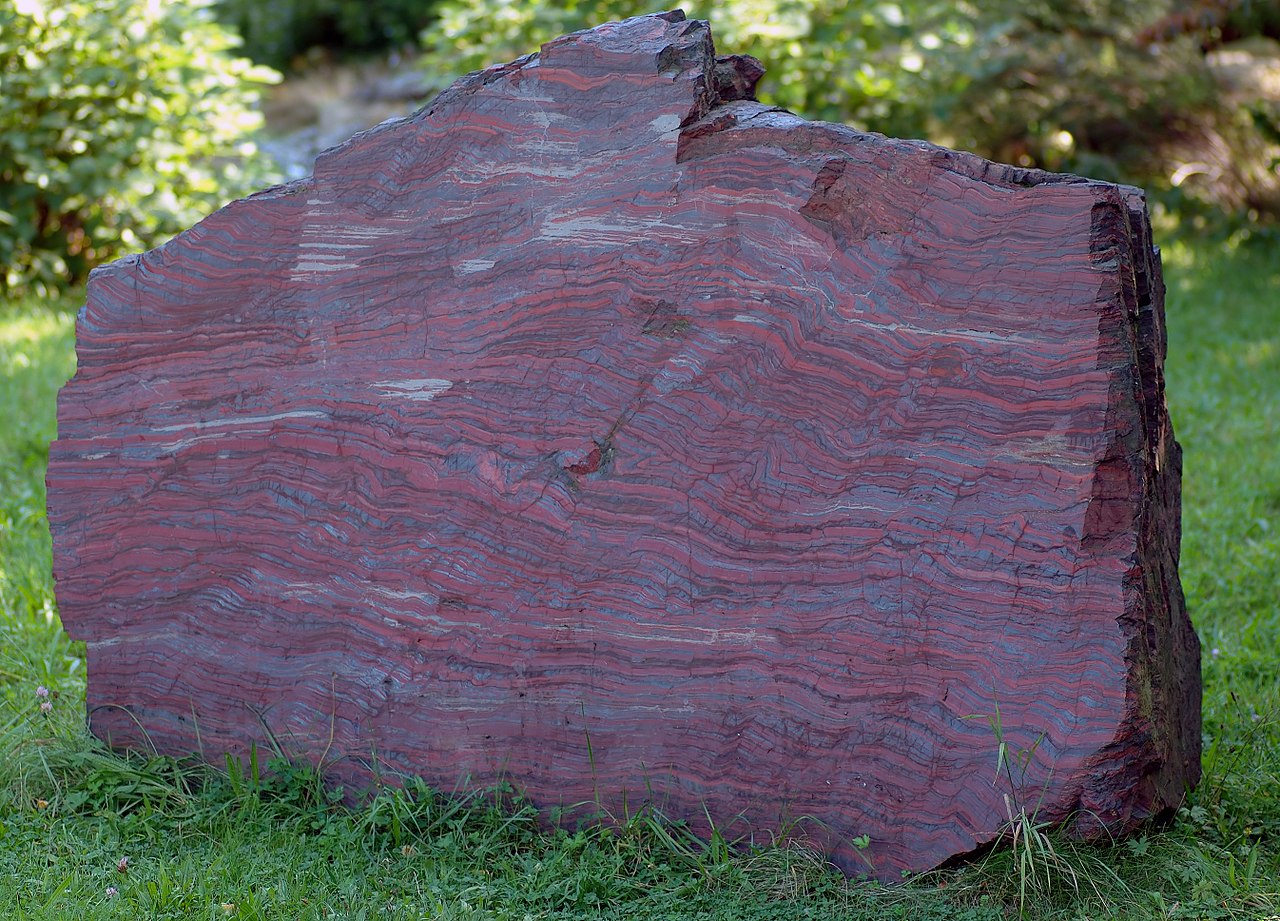
banded iron formation (Chapter 6) an iron-bearing sedimentary rock that is rich in minerals such as hematite and magnetite, which may be interbedded with chert
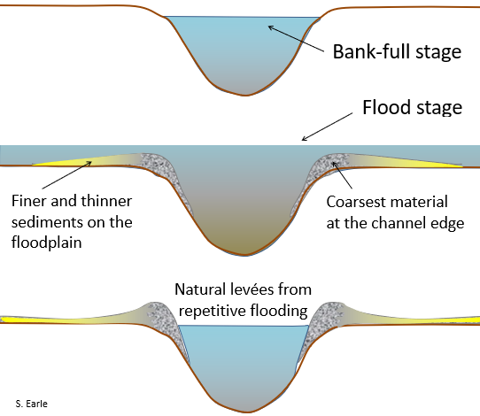
bank-full stage (Chapter 13) the water level of stream when it is in flood and just about to flow over its banks
barrier reef (Chapter 18) a carbonate (or coral) reef that forms a barrier to waves along a coast
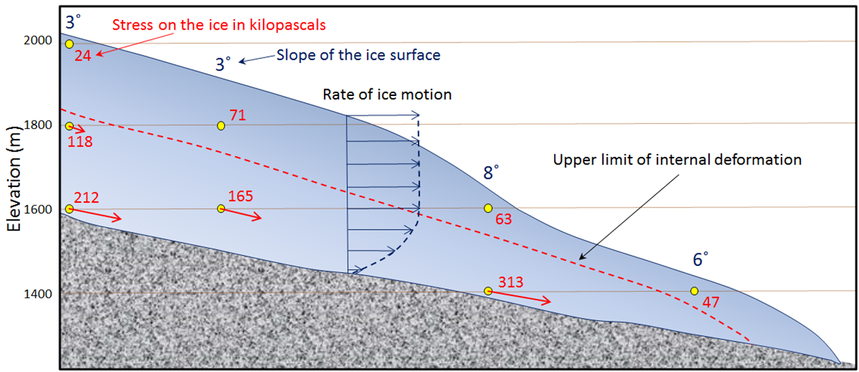
basal sliding (Chapter 16) the motion of glacial ice along the base of a glacier that is warm enough to have liquid water
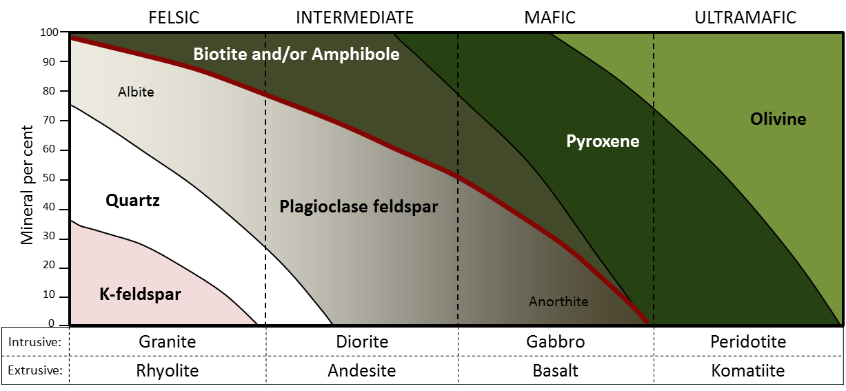
basalt (Chapter 1) a volcanic rock of mafic composition
base level (Chapter 13) in the context of a stream the base level is the lowest level that it can erode down to, as defined by the ocean, a lake or another stream that it flows into
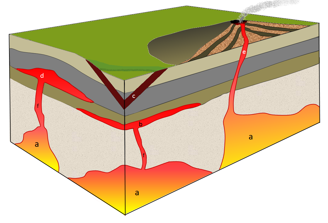
batholith (Chapter 3) an irregular body of intrusive igneous rock that has an exposed surface of at least 100 km2
bathypelagic zone (Chapter 18) the moderately deep parts of the ocean, between 1000 and 4000 metres.
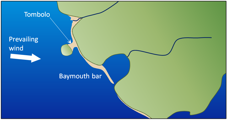
baymouth bar (Chapter 17) a spit that extends across the mouth of a bay
beach face (Chapter 17) the part of the beach that is relatively steep and lies between the high and low tide levels
bed (Chapter 6) a sedimentary layer
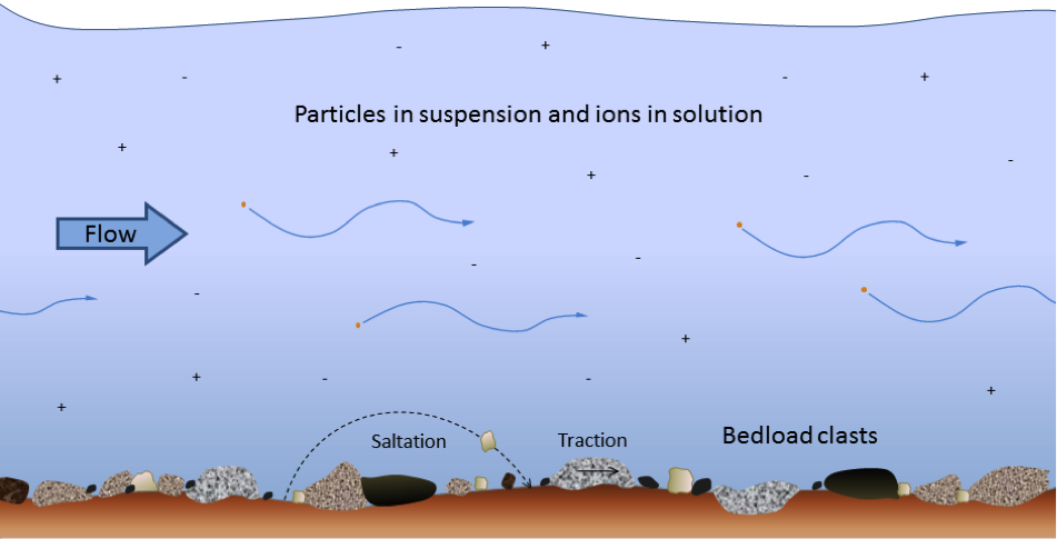
bed load (Chapter 6) the fraction of a stream’s sediment load that typically rests on the bottom and is moved by saltation and traction
bedding (Chapter 6) repeated layering in a sedimentary rock
bentonite (Chapter 15) a type of smectite clay that has strong swelling properties and is effective at absorbing dissolved ions
berm (Chapter 17) a flat area of a beach in the backshore area (above the high tide level)
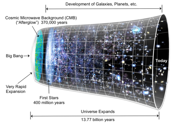
big-bang theory (Chapter 22) the theory that the universe started with a giant explosion approximately 13.77 billion years ago
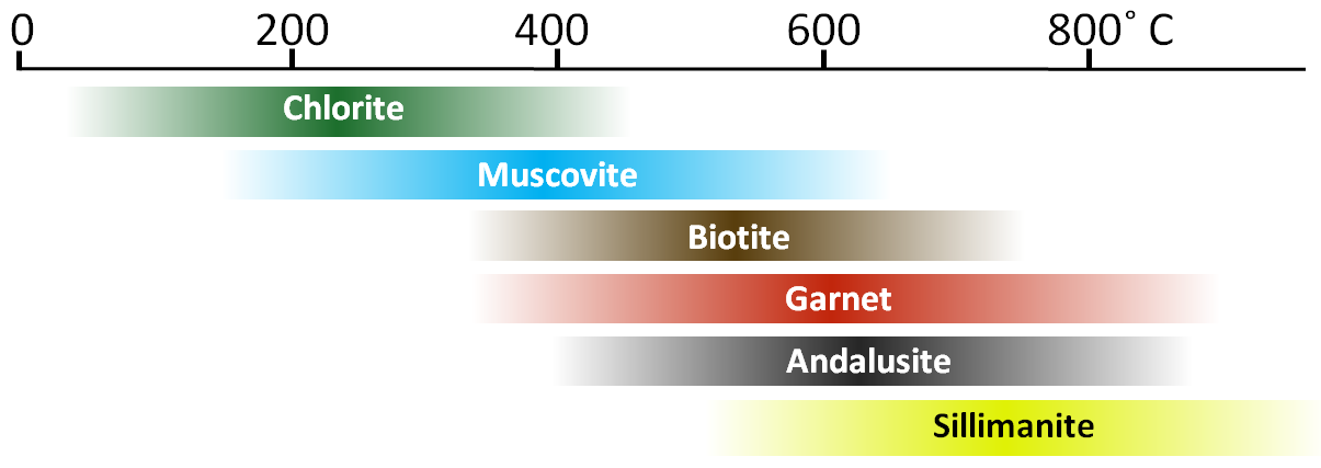
biotite (Chapter 2) a sheet silicate mineral (mica) that includes iron and or magnesium, and is therefore a ferromagnesian silicate
biozone (Chapter 8) a stratigraphic interval that can be defined on the basis of a specific fossil
bituminous (Chapter 20) a medium-grade type of coal with 70 to 92% carbon
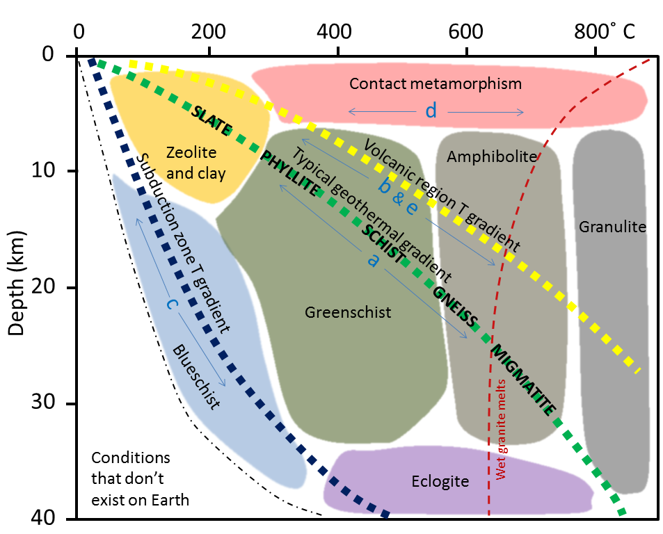
blueschist (Chapter 7) a metamorphic facies characterized by relatively low temperatures and high pressures, such as can exist within a subduction zone
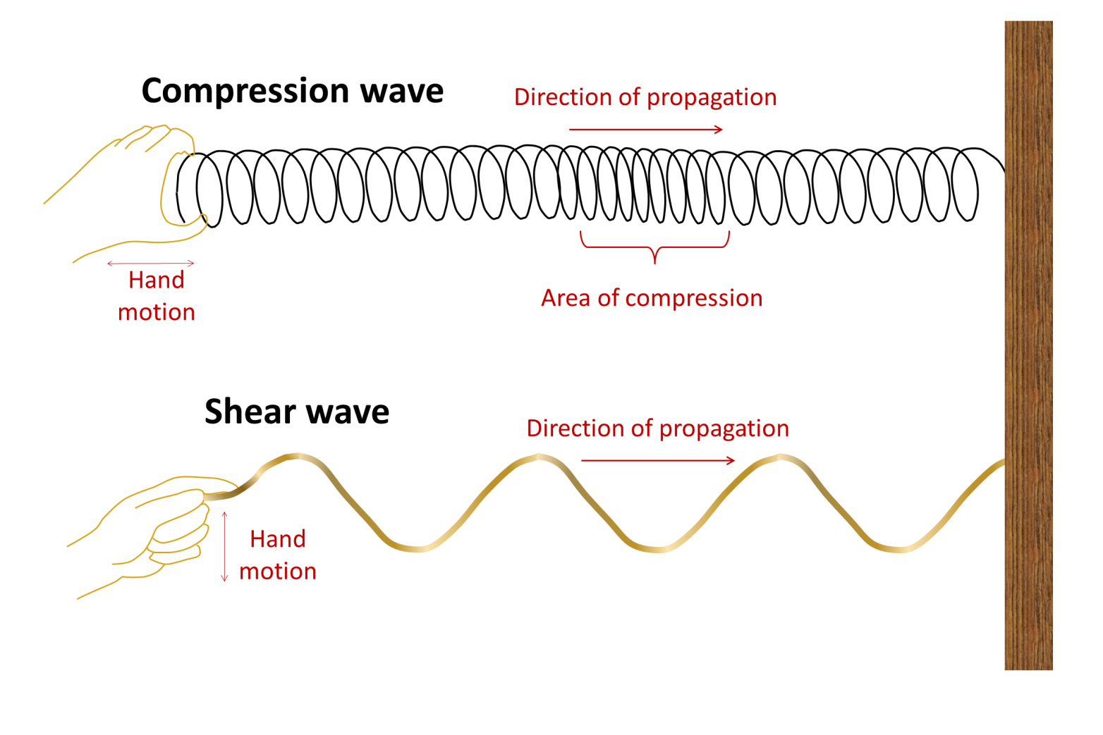
body wave (Chapter 9) a seismic wave that travels through rock (e.g., a P-wave or an S-wave)
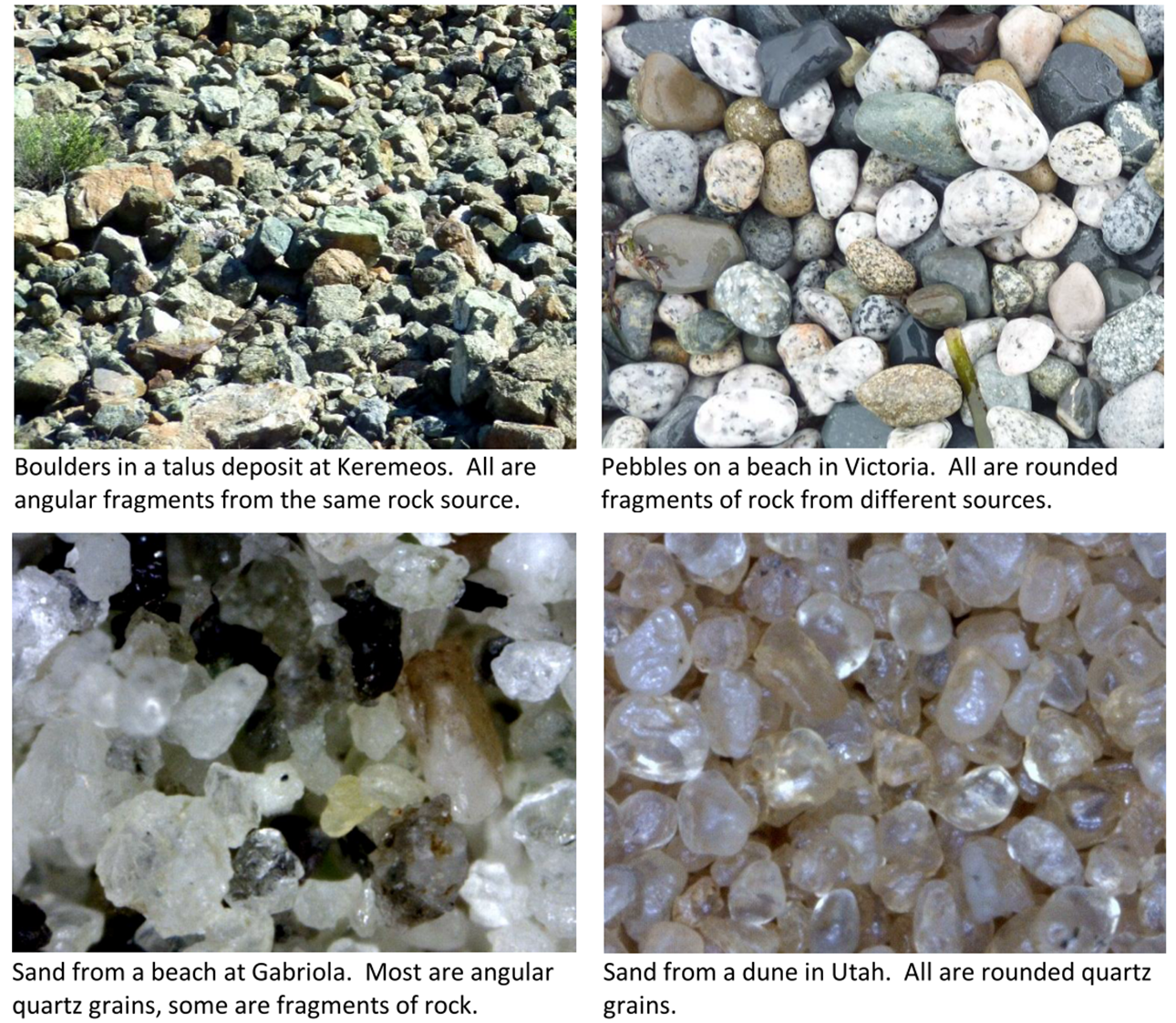
boulder (Chapter 6) a sediment clast with a diameter of at least 256 millimetres
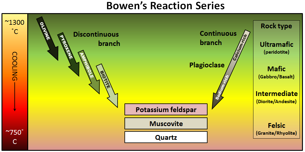
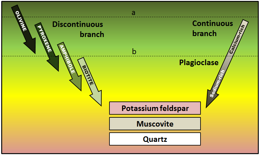
Bowen reaction series (Chapter 3) the scheme that defines the typical order of crystallization of minerals from magma
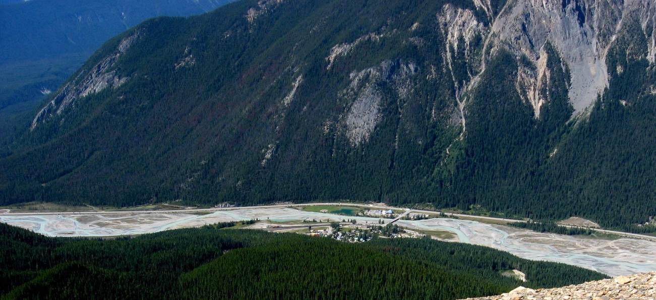
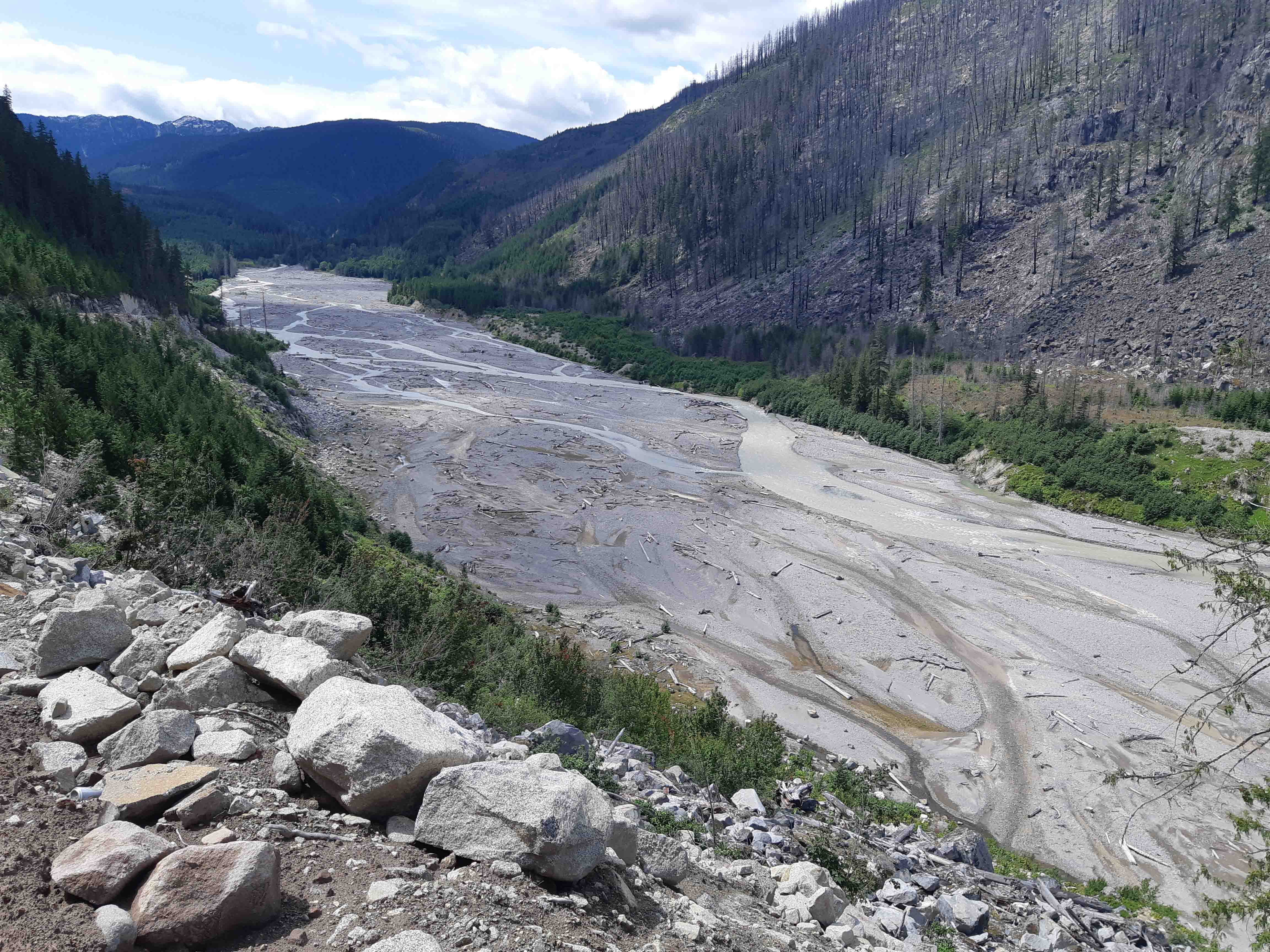
braided (Chapter 13) a stream pattern which is characterized by abundant sediment and numerous intertwining channels around bars
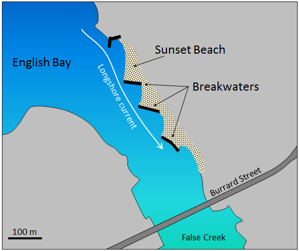
breakwater (Chapter 17) a structure built offshore in order to deflect the energy of waves
breccia (Chapter 6) a sedimentary- or volcanic-rock texture characterized by angular clasts
brunisol (Chapter 5) a relatively immature forest soil, lacking in well-defined horizons
C
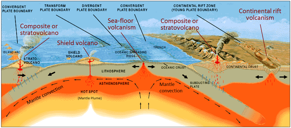
caldera (Chapter 4) a volcanic depression that is many times larger than the volcanic vents within it
caliche (Chapter 5) a white calcium-carbonate rich layer within soils in arid regions
calving (Chapter 16) the loss of ice from the front of a glacier by collapse into water
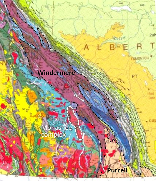
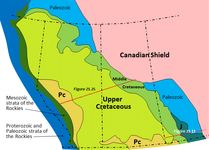
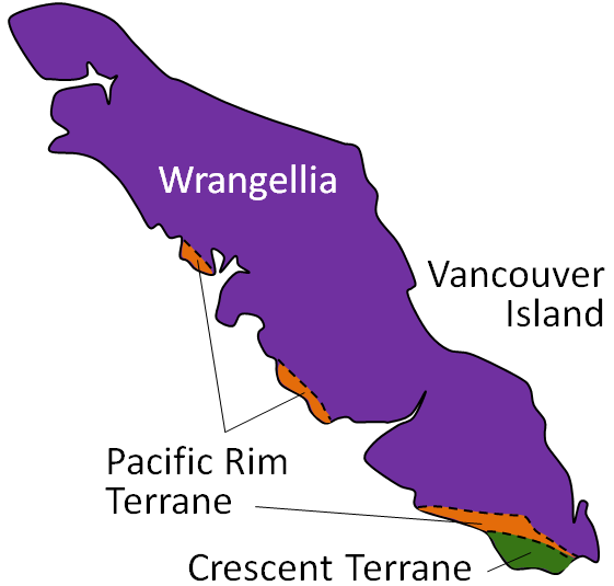
Canadian Shield (Chapter 21) the exposed part of the continent Laurentia
carbonate (Chapter 2) a mineral in which the anion is CO3-2
carbonate compensation depth (Chapter 18) the depth in the ocean (typically around 4000 metres) below which carbonate minerals are soluble
cation (Chapter 2) a positively charged ion
cementation (Chapter 6) the process by which minerals are precipitated between grains in sediments
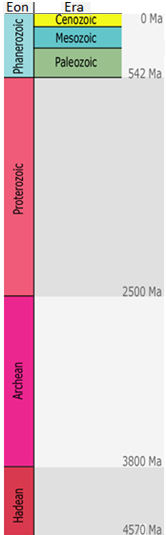
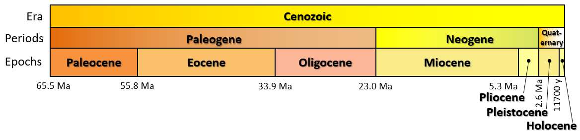
Cenozoic (Chapter 1) the most recent of the eras, representing the past 65.5 Ma of geological time
chemical sedimentary rock (Chapter 6) a sedimentary rock comprised of material that was transported as ions in solution
chernozem (Chapter 5) a black soil typical of grasslands in cold climates such as the Canadian Prairies
chert (Chapter 6) a very fine grained sedimentary rock formed almost entirely of silica
chlorite (Chapter 2) a ferromagnesian sheet silicate mineral, typically present as fine crystals and forming from the low-temperature metamorphism of mafic rock
cinder cone (Chapter 4) a steep-sided volcano comprised almost entirely of loose rock fragments and typically formed during a single eruptive event
cirque (Chapter 16) a steep-sided semi-circular basin eroded by a glacier at the head of its valley
clast (Chapter 6) a sedimentary fragment of mineral or rock
clastic sedimentary rock (Chapter 6) a sedimentary rock comprised of material that was transported as clasts or fragments
clay (Chapter 6) sediment particle that is less than 1/256 millimetres in diameter
clay mineral (Chapter 6) a hydrous sheet silicate mineral that typically exists as clay-sized grains
claystone (Chapter 6) a sedimentary rock comprised mostly of clay-sized grains
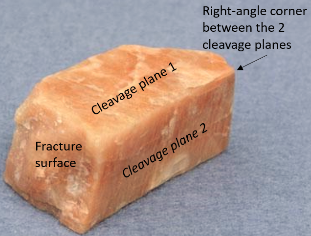
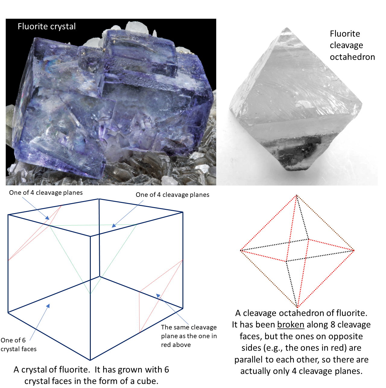
cleavage (Chapter 2) the tendency for a mineral to break along smooth planes that are predetermined by its lattice structure
climate feedback (Chapter 19) a process by which the physical effects of a climate forcing can have other effects (either negative or positive) on the climate
climate forcing (Chapter 19) a mechanism, such as a change in greenhouse gas levels, that forces the climate to change
coal-bed methane (Chapter 20) methane that is trapped within the porosity of coal
coastal straightening (Chapter 17) the tendency for an irregular coast to be straightened over time by coastal erosion processes
cobble (Chapter 6) sediment particle that is between 64 and 256 millimetres in diameter
col (Chapter 16) the low point or pass along a ridge between two glacial valleys
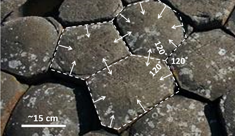
columnar jointing (Chapter 4) the fracturing of rock or sediment (but typically volcanic rock) into columns that are typically six-sided
composite volcano (or stratovolcano) (Chapter 4) a volcano that is constructed of alternating layers of pyroclastic debris and lava flows
concentrate (mining) (Chapter 20) a product of ore processing that includes a specific ore mineral, separated from the rest of the rock
concordant (Chapter 3) parallel to pre-existing layering or foliation within a rock
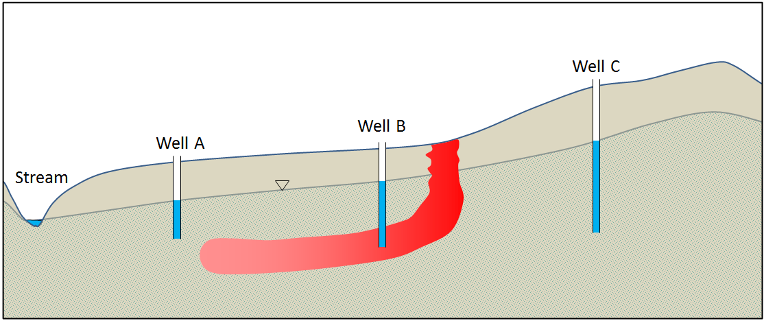
cone of depression (Chapter 14) the depression of the water table around a well that is heavily pumped
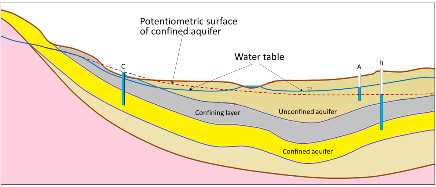
confined aquifer (Chapter 14) an aquifer that lies below a confining layer
confining layer (Chapter 14) an aquitard that overlies an aquifer and restricts the flow of water down from the surface
conglomerate (Chapter 6) a sedimentary rock that is comprised predominantly of rounded grains that are larger than 2 mm
contact metamorphism (Chapter 7) metamorphism that takes place adjacent to a source of heat, such as a body of magma
continental drift (Chapter 10) the concept that tectonic plates can move across the surface of the Earth
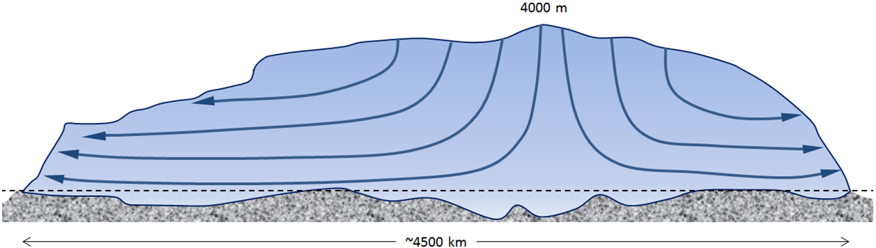
continental glacier (Chapter 16) a glacier that covers a significant part of a continent and has an area of at least 50,000 km2
continental shelf (Chapter 18) the shallow (typically less than 200 metres) and flat sub-marine extension of a continent
continental slope (Chapter 18) the steeper part of a continental margin, that slopes down from a continental shelf towards the abyssal plain
contractionism (Chapter 10) the now discredited theory that mountain ranges formed as a result of the contraction of the Earth
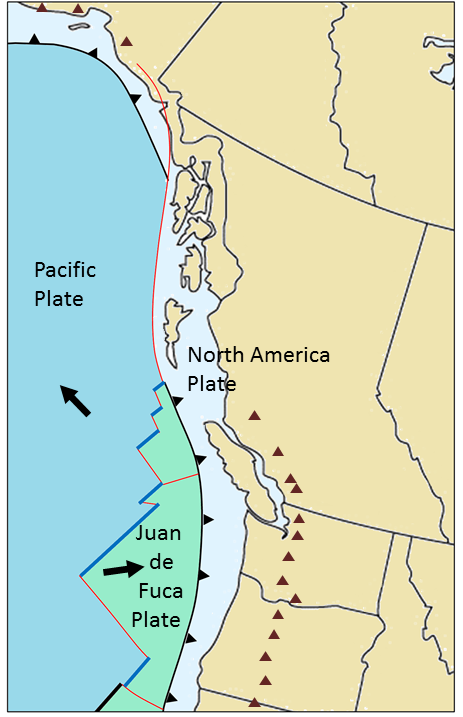
convergent boundary (Chapter 10) a plate boundary at which the two plates are moving towards each other
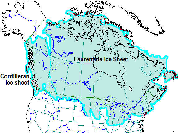
Cordilleran Ice Sheet (Chapter 16) the continental glacier that covered part of western North America, including almost all of British Columbia, part of the Yukon, and part of northern Washington, during the Pleistocene glaciations
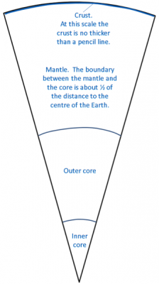
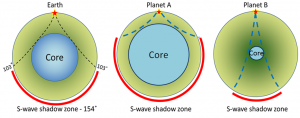
core (Chapter 1) the metallic interior part of the Earth, extending from a depth of 2900 kilometres to the centre
core-mantle boundary (Chapter 9) the boundary, at a 2900 kilometre depth, between the mantle and the core
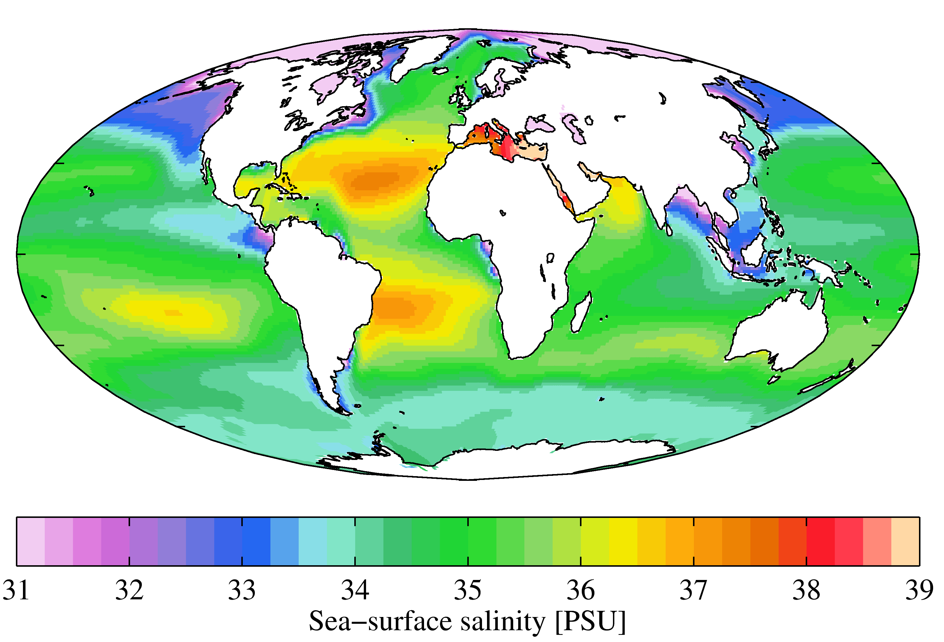
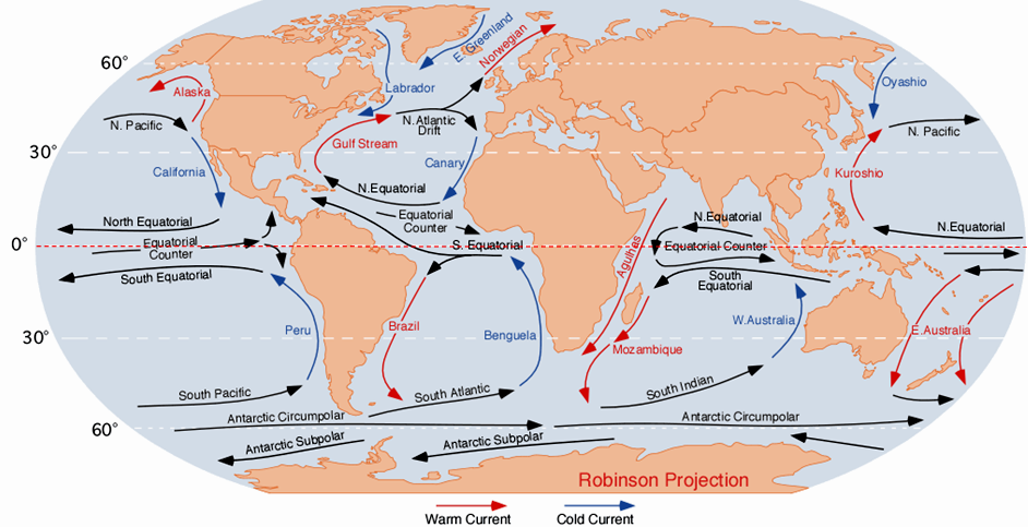
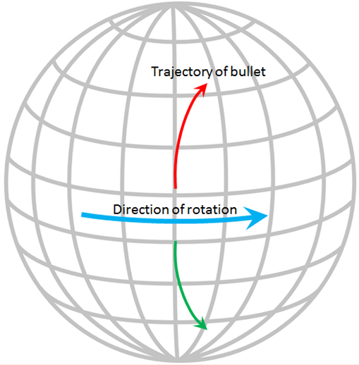
Coriolis effect (Chapter 18) the tendency for moving bodies (e.g., ocean currents) to rotate on the surface of the Earth, clockwise in the northern hemisphere and counter-clockwise in the southern hemisphere
cosmic microwave background (Chapter 22) radiation left over from the an early stage in the development of the universe at the time when protons and neutrons were recombining to form atoms
country rock (Chapter 3) the original rock of a region, into which younger rock (typically igneous) rock has been intruded
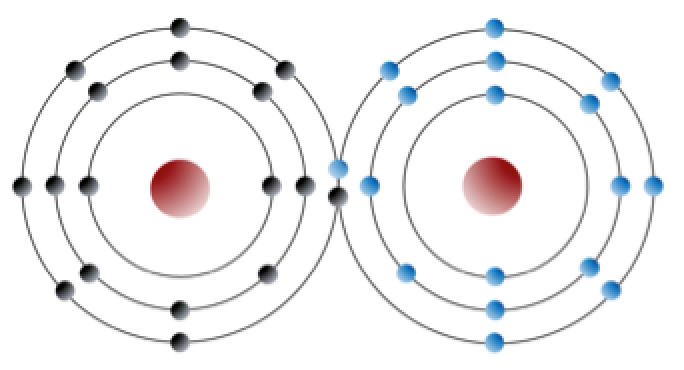
covalent bond (Chapter 2) a bond between two atoms in which electrons are shared
crater (Chapter 4) a volcanic depression that is related to a specific volcanic vent
craton (Chapter 21) a region of ancient (typically Precambrian) crystalline rock (equivalent to a shield)
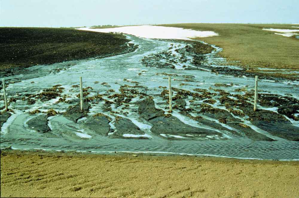
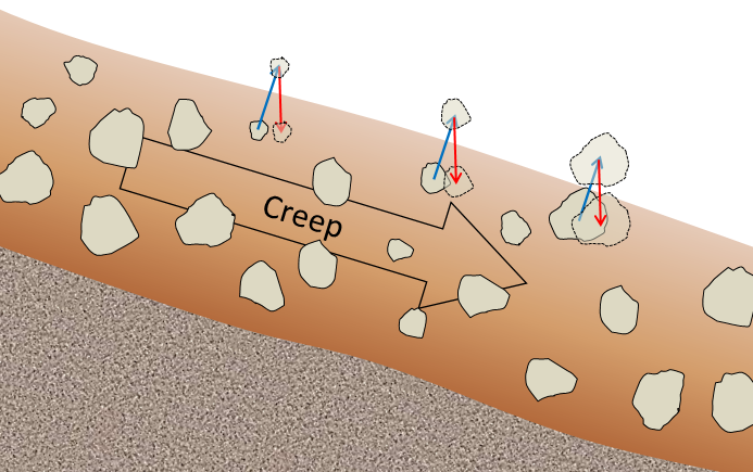
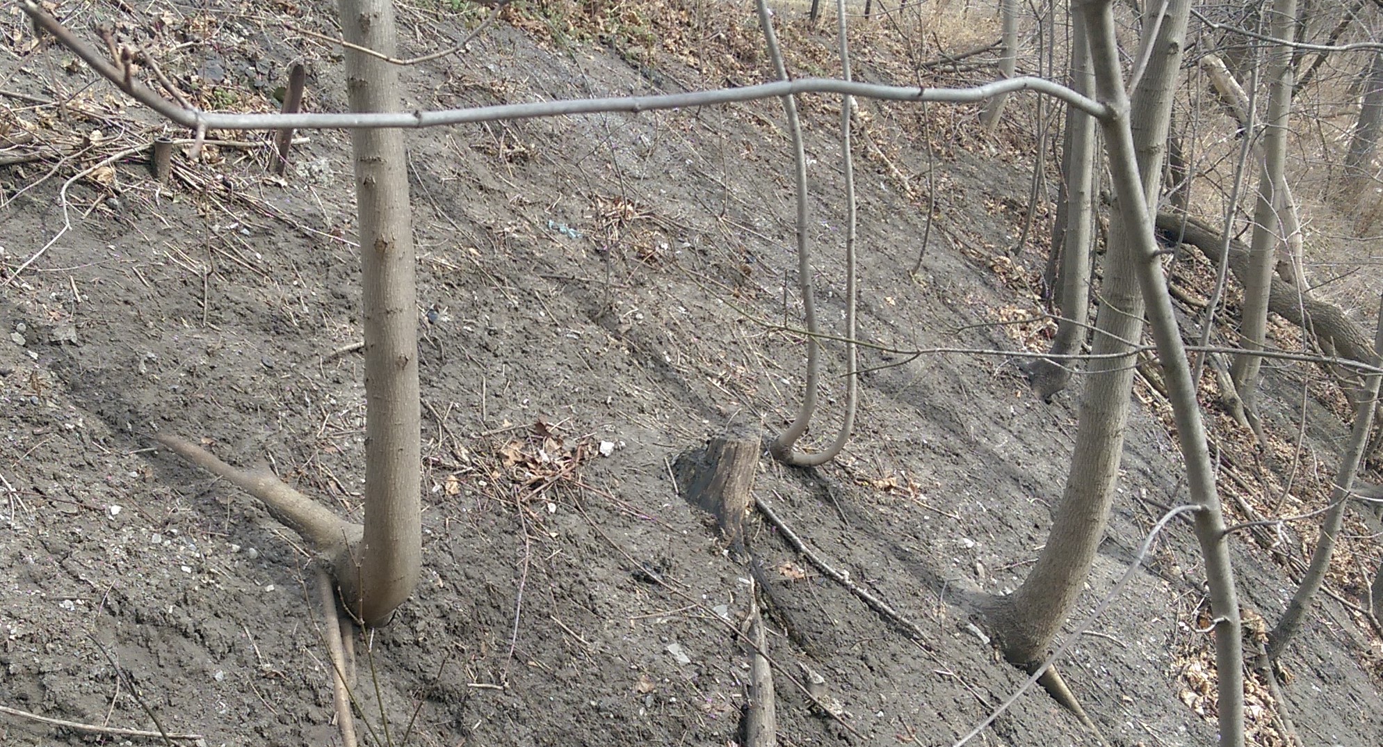
creep (Chapter 15) the very slow (a millimetre to centimetre per year) flow of unconsolidated material on a gentle slope
crest (Chapter 17) the highest point on a wave
crevasse (Chapter 16) an open fissure on the surface of a glacier
cross bedding (Chapter 6) small-scale inclined bedding within larger horizontal beds
crust (Chapter 1) the uppermost layer of the Earth, ranging in thickness from about 5 kilometres (in the oceans) to over 50 kilometres (on the continents)
cyanobacteria (Chapter 6) photosynthetic bacteria that evolved in the early Archean
D
“D” layer (Chapter 9) (d-double-prime layer) a low seismic velocity zone within the basal 200 km of the mantle
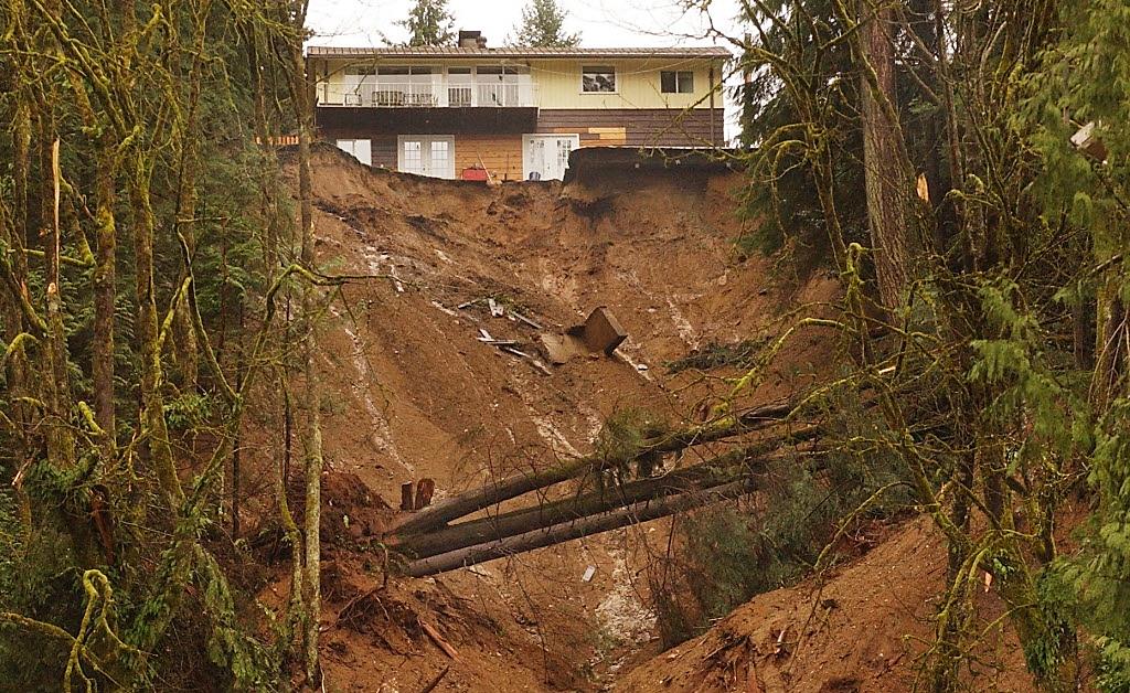
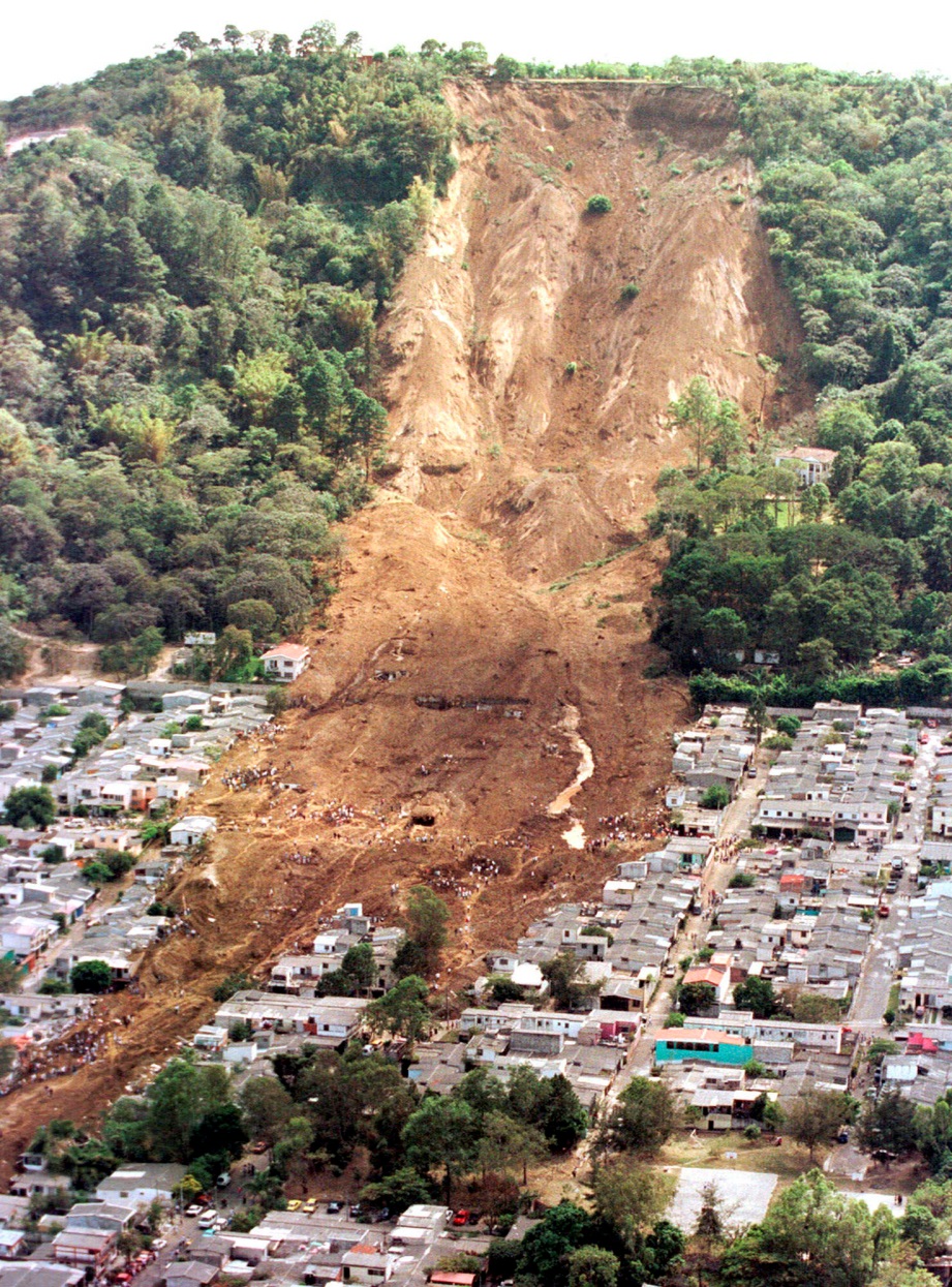
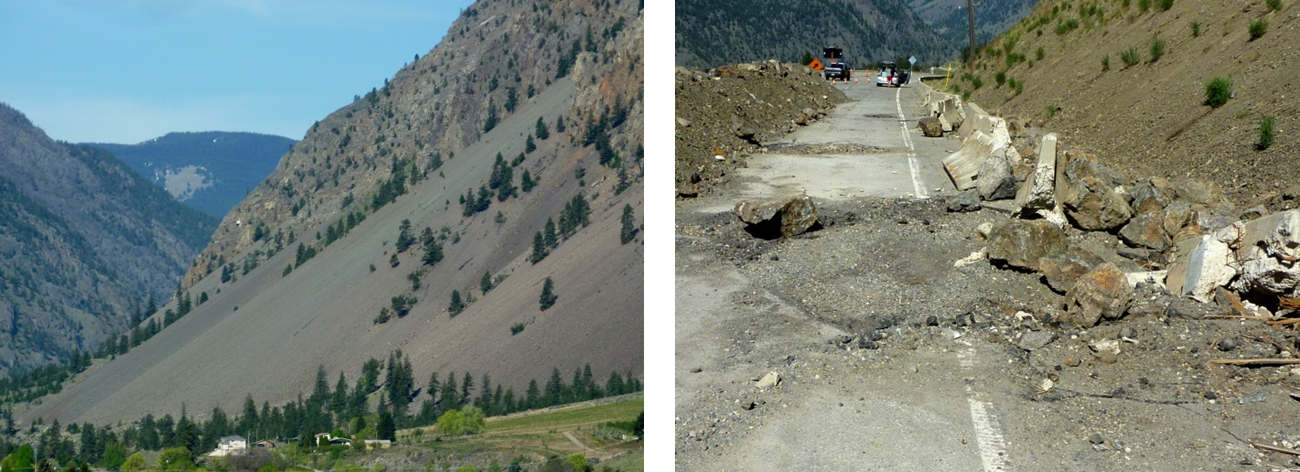
debris flow (Chapter 15) a gravity-driven flow of water and sediment that includes a significant proportion of coarse (cobble to boulder) material
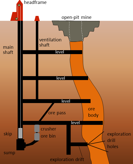
decline (Chapter 20) in mining a decline is a sloped tunnel used to access lower parts of a mine with wheeled equipment
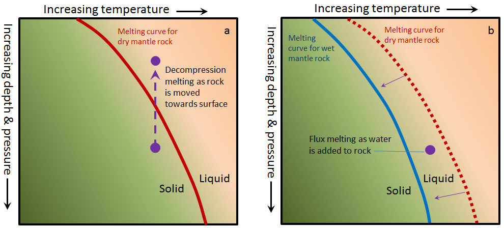
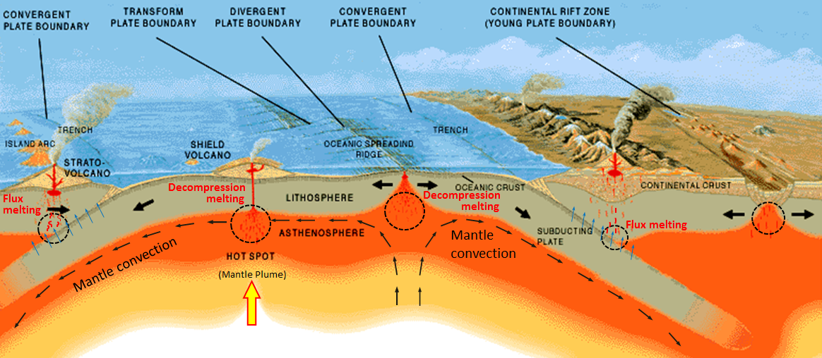
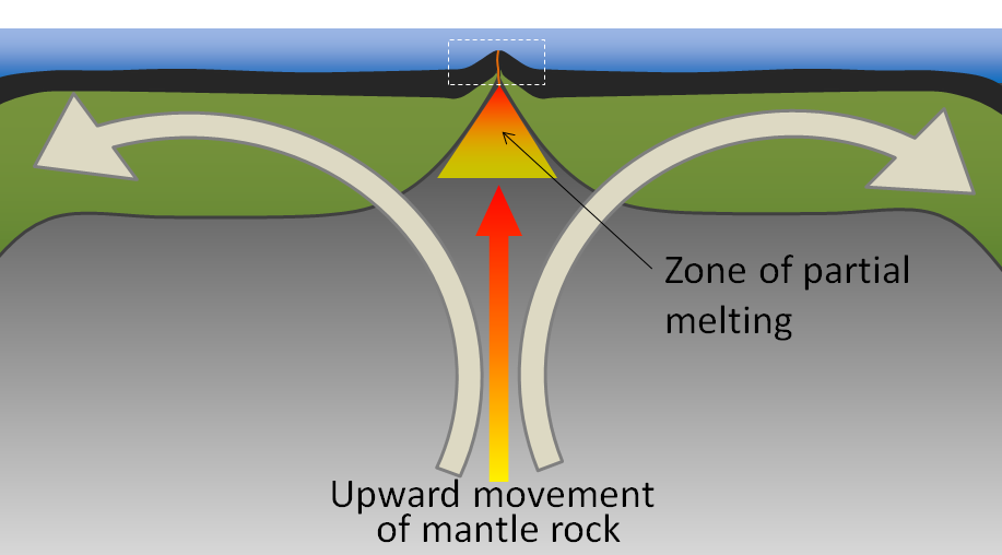
decompression melting (Chapter 3) melting (or partial melting) of rock resulting from a reduction in pressure without a significant reduction in temperature
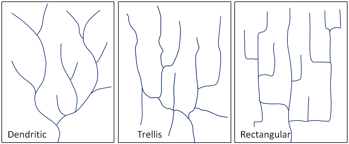
dendritic (Chapter 13) a pattern of drainage channels that resembles the branches in a tree
density (Chapter 2) weight per volume of a substance (e.g., g/cm3) used widely in the context of minerals or rocks
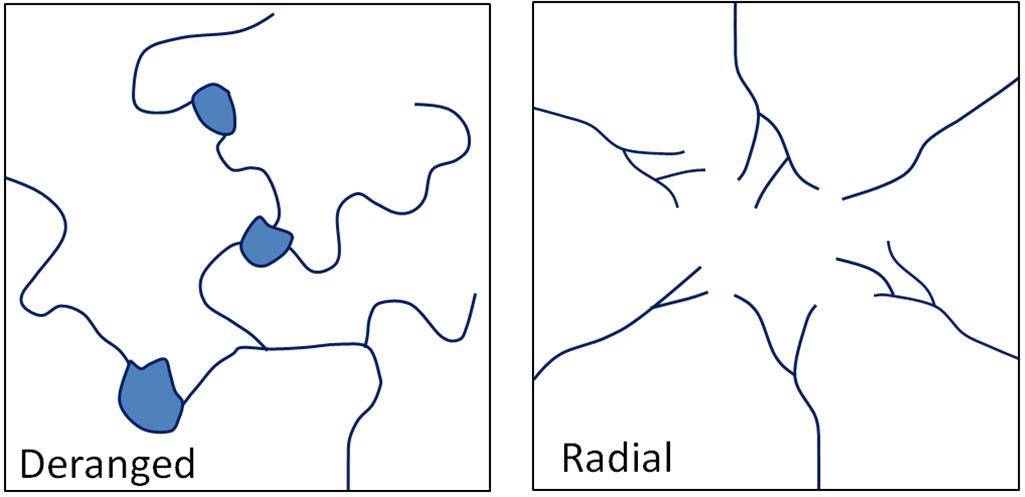
deranged (Chapter 13) a pattern of drainage channels that is chaotic
detrital (Chapter 6) referring to fragments of rocks or minerals
diatom (Chapter 18) photosynthetic algae that make their tests (shells) from silica
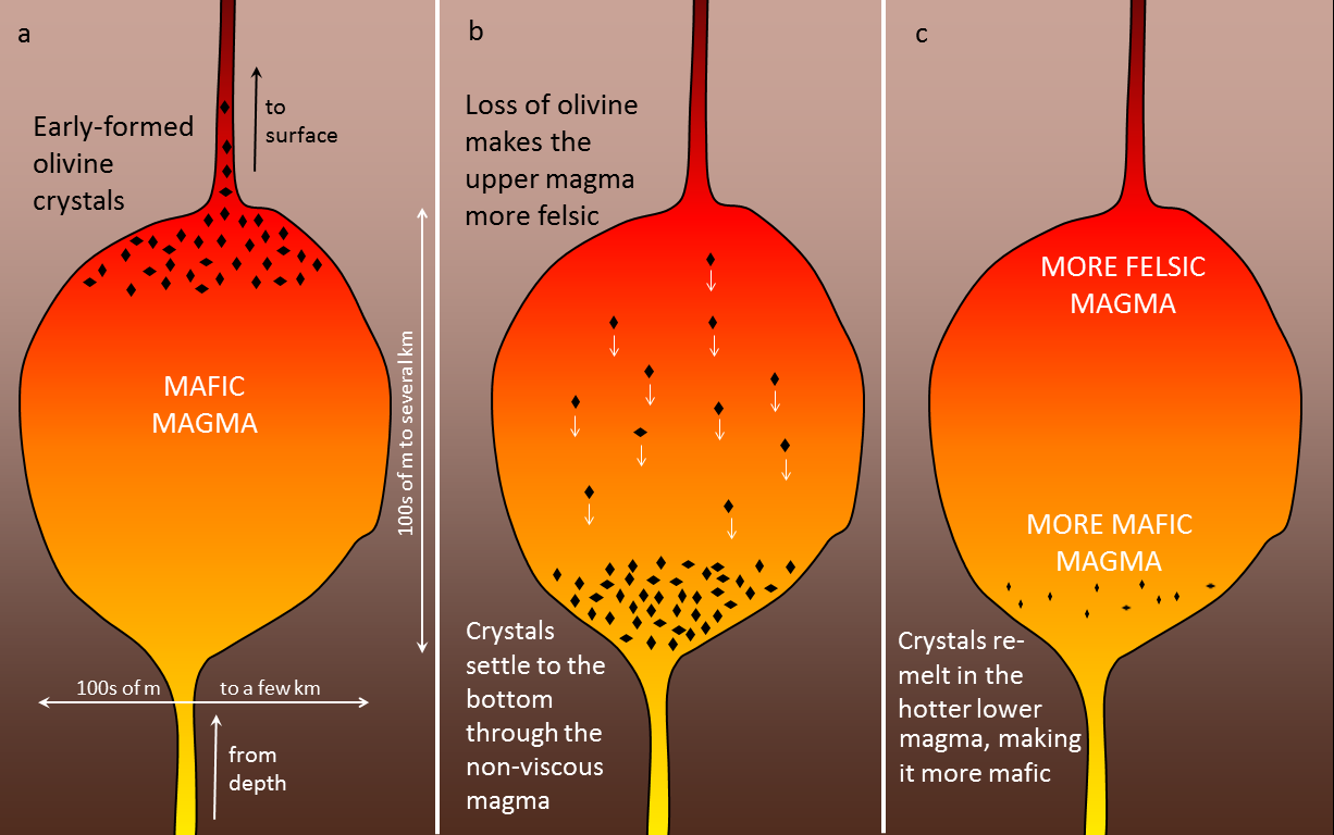
differentiation (Chapter 22) the un-mixing of a magma, typically by the physical separation of minerals that crystallize early and settle towards the bottom
diorite (Chapter 3) an intermediate intrusive igneous rock
dip (Chapter 12) the angle below horizontal at which a sedimentary bed or other feature slopes
discharge (Chapter 6) the volume of water flow in a stream expressed in terms of volume per unit time (e.g., m3/s)
discharge area (Chapter 14) the part of an aquifer where groundwater discharge takes place
disconformity (Chapter 8) a boundary between parallel sedimentary layers where some erosion of the lower layer has taken place
discordant (Chapter 3) a geological feature that is not parallel to any existing layering in the country rock
divalent (Chapter 2) an ion with a charge or +2 or -2
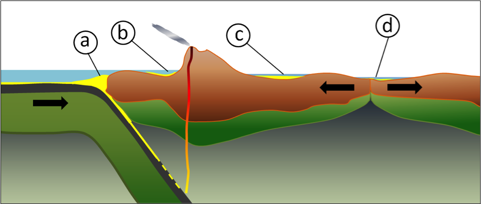
divergent (Chapter 10) a plate boundary at which the two plates are moving towards away from each other
dodecahedron (Chapter 2) an object with twelve surfaces, such as a garnet crystal
dolomite (Chapter 6) a calcium-magnesium carbonate mineral (Ca,Mg)CO3
dolomitization (Chapter 6) the addition of magnesium to limestone during which some or all of the calcium carbonate is converted to dolomite
dolostone (Chapter 6) a carbonate rock made up primarily of the mineral dolomite
drainage basin (Chapter 13) the catchment area of a stream, including the area where all surface water drains into the stream
drop stone (Chapter 16) a fragment of rock within otherwise fine-grained sediment that has been dropped from floating ice on a body of water
drumlin (Chapter 16) a streamlined glacial erosional feature comprised of sediments and/or bedrock
dyke (Chapter 3) a tabular intrusive igneous body that is discordant to any existing layering in the country rock
E
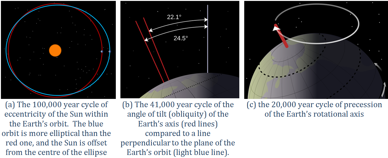
eccentricity (Chapter 19) in the context of Milankovitch Cycles, the degree to which the Sun is offset from the geometric centre of the Earth’s orbit
eclogite (Chapter 7) a garnet-pyroxene-glaucophane bearing rock that is the product of high-pressure metamorphism of oceanic crustal rock, typically within a subduction zone
effusive (Chapter 4) a volcanic eruption dominated by the relatively gentle flow of lava
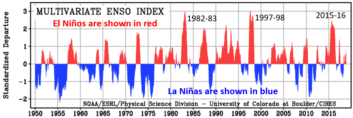
El Niño (Chapter 19) a periodic climatic situation in which warm water extends all or most of the way to the eastern edge of the equatorial Pacific
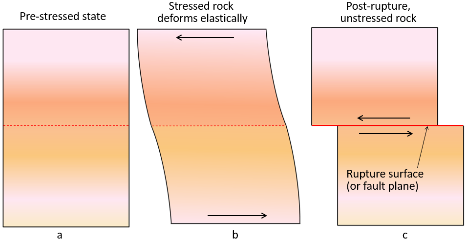
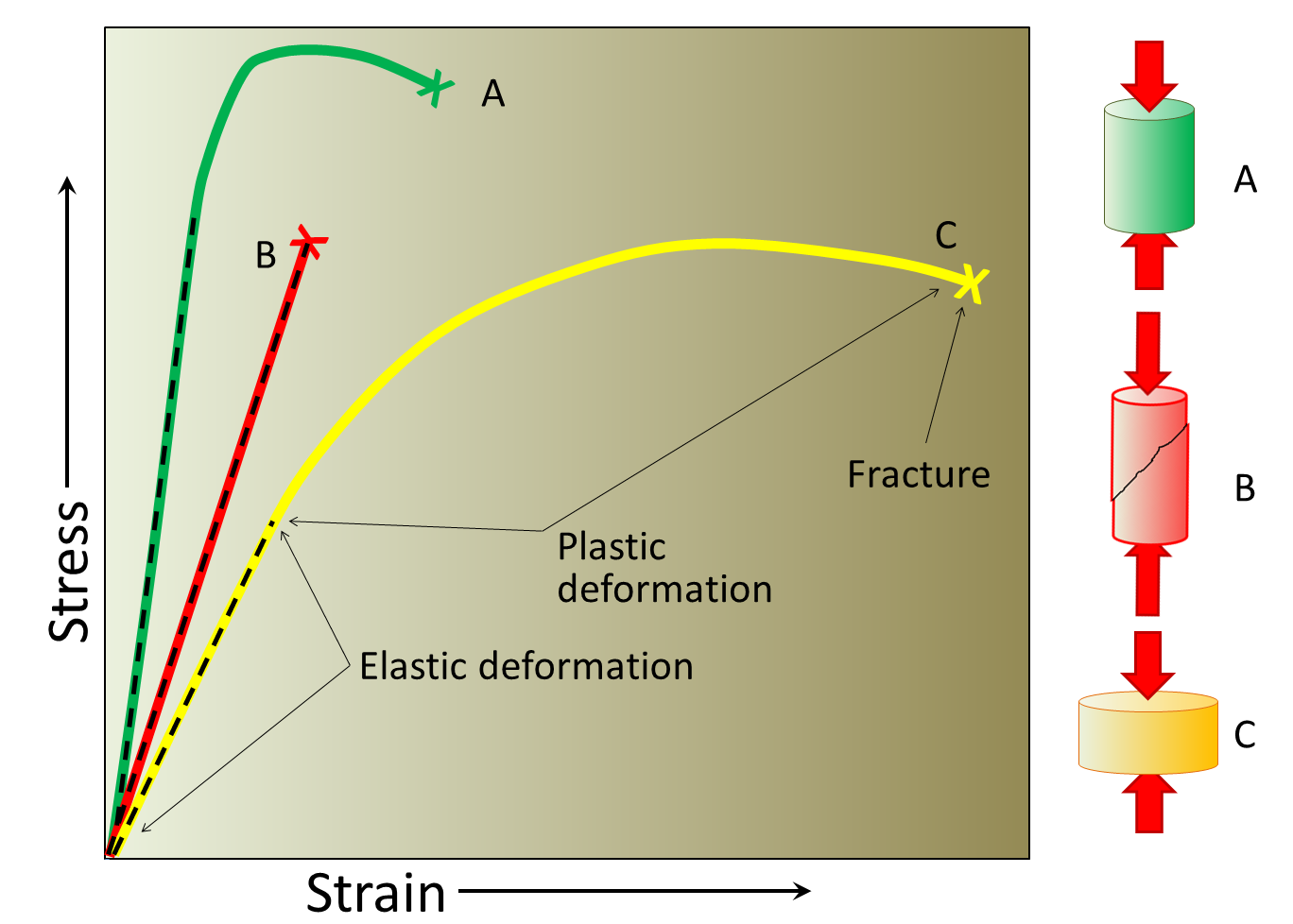
elastic deformation (Chapter 11) the deformation of material (including rock) from which it can fully recover if the stress is removed
electron (Chapter 2) a sub-atomic particle of essentially no mass and a single negative charge
end moraine (Chapter 16) a deposit of sediment that accumulates at the front of a glacier
englacial (Chapter 16) within a glacier, referring especially to sediment carried within the glacial ice
epicentre (Chapter 11) the location on the surface vertically above the location (i.e., “hypocentre” or “focus”) where an earthquake takes place
epipelagic zone (Chapter 18) the upper layer of water (0 to 200 metres) in areas of the open ocean
epithermal deposit (Chapter 20) a mineral deposit formed near to surface in an area of hydrothermal activity, typically associated with a body of magma
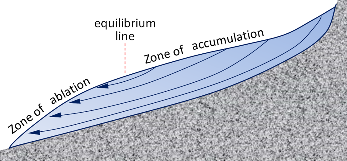
equilibrium line (Chapter 16) on a glacier, the line between the zone of accumulation and the zone of ablation (in late summer the equilibrium line is the boundary between snow-covered ice and bare ice)
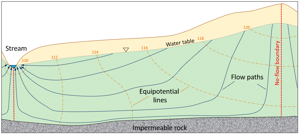
equipotential lines (Chapter 14) in the context of groundwater an equipotential line connects locations with equal hydraulic head or water pressure
esker (Chapter 16) a ridge of sediment deposited by a sub-glacial stream
eustatic sea level change (Chapter 17) sea level change related to a change in the volume of the oceans, typically because of an increase or decrease in the amount of glacial ice on land
exfoliation (Chapter 5) the fracturing of rock that results from a reduction in the pressure when overlying rock is eroded away
exoplanet (Chapter 22) a planet that orbits a star other than the Sun
extrusive (Chapter 3) igneous rock that cooled at surface
F
fall (Chapter 15) in mass wasting, the vertical or near-vertical fall of rock
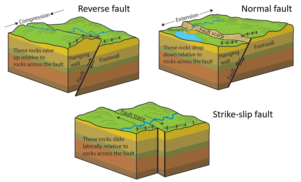
fault (Chapter 12) a boundary in rock or sediment along which displacement has taken place
feedback (Chapter 19) a process by which the physical effects of a climate forcing can have other effects (either negative or positive) on the climate
feldspar (Chapter 2) a very common framework silicate mineral
felsic (Chapter 3) silica rich (>65% SiO2) in the context of magma or igneous rock
ferric (Chapter 2) the oxidized form of an ion of iron (Fe3+)
ferromagnesian (Chapter 2) referring to a silicate mineral that contains iron and or magnesium
ferrous (Chapter 2) the reduced (non-oxidized) form of an ion of iron (Fe2+)
fetch (Chapter 17) the distance over which wind blows to form waves
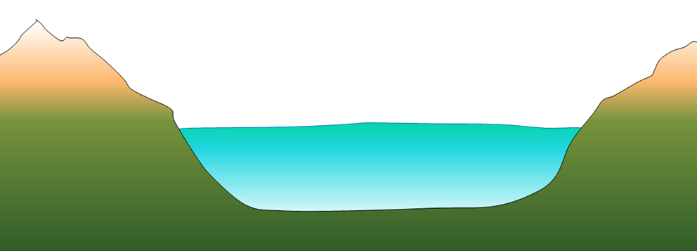
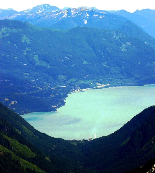
finger lake (Chapter 16) a lake that occupies a glacial valley
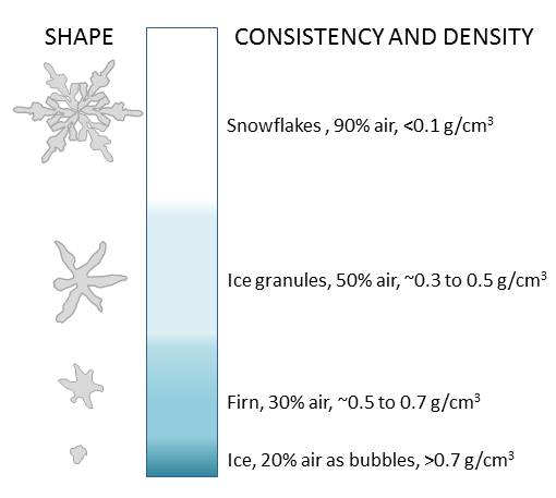
firn (Chapter 16) the granular transitional state between snow and ice within a glacier
flood plain (Chapter 13) the area that is occupied by water when a stream floods and overtops its banks
flow (Chapter 15) the fluid-like motion of material during mass-wasting
flow path (Chapter 14) the path that groundwater flows along between a recharge area and a discharge area
flowing artesian well (Chapter 14) an artesian well in which the water level naturally rises above the surface of the ground
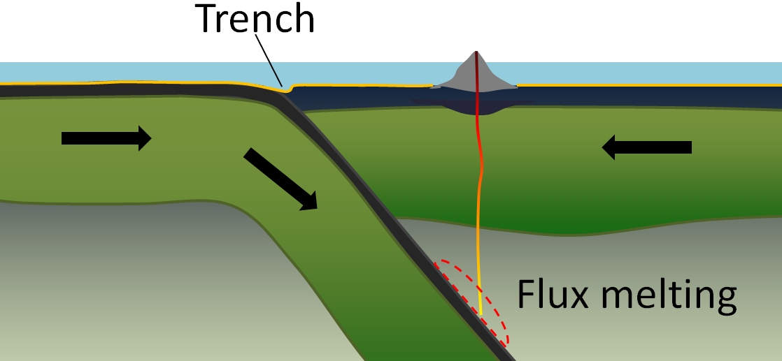
flux melting (Chapter 3) melting of rock that is facilitated by the addition of a flux (typically water) which lowers the rocks melting point
focus (earthquake) (Chapter 11) the actual point below surface at which an earthquake takes place (equivalent to hypocentre)
foliated (Chapter 7) the existence of foliation in a metamorphic rock
foliation (Chapter 7) the alignment of mineralogical or structural features of a rock – especially a metamorphic rock
(Chapter 12) the lower surface of a non-vertical fault
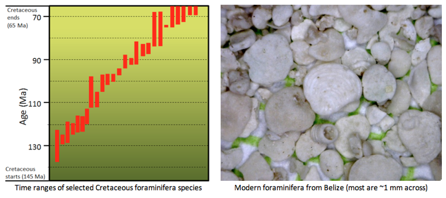
foraminifera (Chapter 18) a single-celled protist with a shell that is typically made of CaCO3
fore-reef (Chapter 6) the zone on the ocean side of a reef
formation (Chapter 6) a unit of sedimentary rock that is lithologically consistent and sufficiently thick and extensive to be shown on a geological map at the scale that is typically used in the area in question
fracking (Chapter 20) fracturing rock by injecting water and chemicals down a well at very high pressure (equivalent to hydraulic fracturing)
fractional crystallization (Chapter 3) the sequential crystallization of minerals from magma, and the physical separation of early-forming crystals from the magma in the area where they crystallized
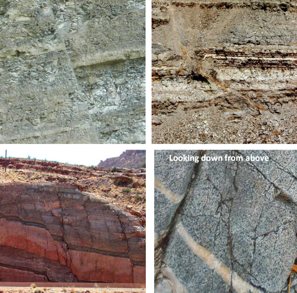
fracture (Chapter 2) a break within a body of rock in which the rock on either side is not displaced
fringing reef (Chapter 18) a reef adjacent to a shoreline where there is either a very narrow back reef area or none at all (in which case the reef is effectively attached to the shore)
frost line (Chapter 22) in the context of planetary systems the boundary beyond which volatile components (e.g., water, carbon dioxide, methane, ammonia etc.) are frozen
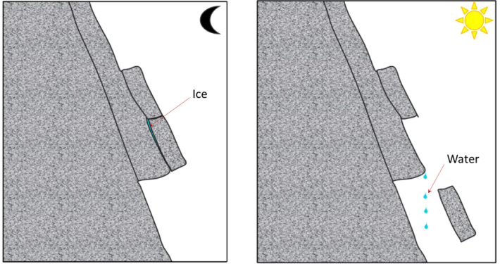
frost wedging (Chapter 5) the situation where the expansion of freezing water pries rock apart
G
Ga (Chapter 1) (giga annum) billions of years before the present
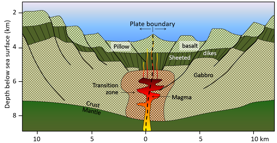
gabbro (Chapter 3) a mafic intrusive igneous rock
Gaia hypothesis (Chapter 19) the hypothesis advanced by James Lovelock that the organisms have affected the atmosphere and oceans such that conditions on Earth have been kept habitable, in spite of significantly changing energy received from the Sun
galaxy (Chapter 22) a gravitationally-bound system of stars and interstellar matter
gas giant (Chapter 22) a large planet composed mostly of hydrogen and helium (e.g. Jupiter)
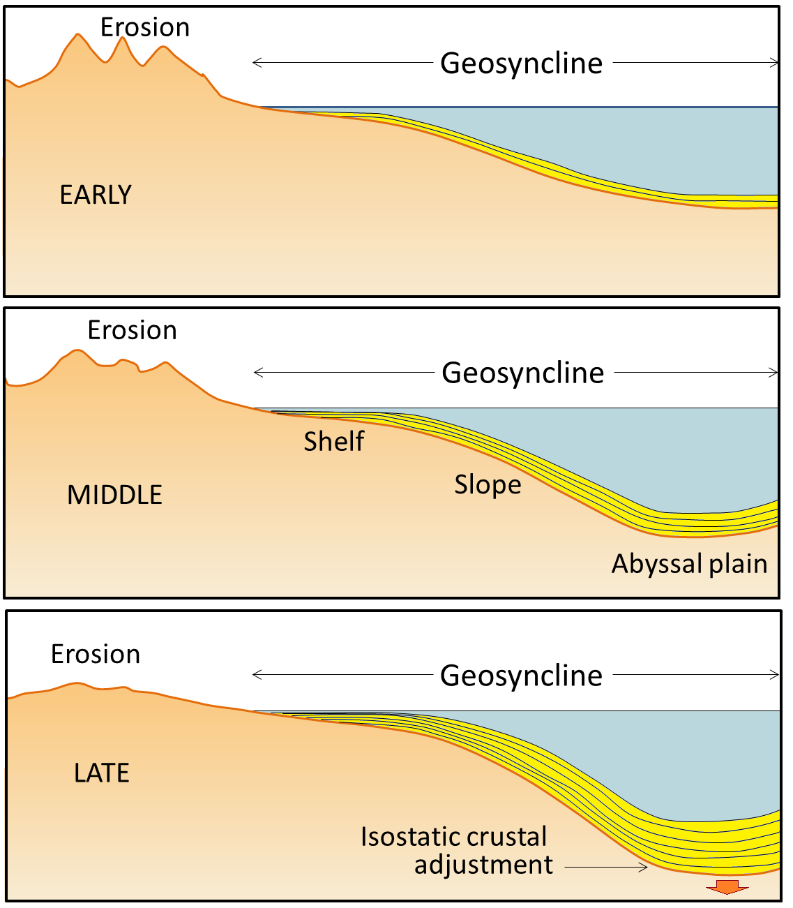
geosyncline (Chapter 10) a kilometre thick deposit of sediments that has accumulated along the edge of a continent and is sufficient mass to depress the crust beneath it
geothermal gradient (Chapter 1) the rate of increase of temperature with depth in the Earth (typically around 30˚ C/km within the crust)
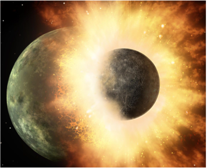
giant impact hypothesis (Chapter 22) the theory that the Moon formed when a Mars-sized planet (Theia) collided with the Earth at 4.5 Ga
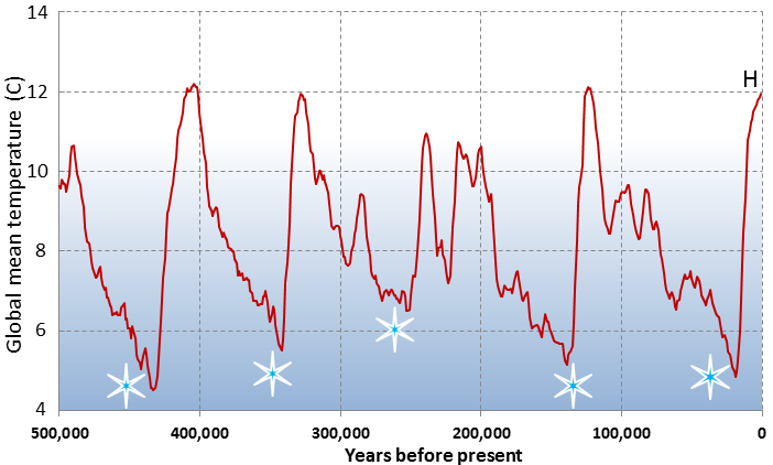
glacial period (Chapter 16) a period of Earth’s history during which glacial ice was present over a sufficient extent to have left recognizable evidence
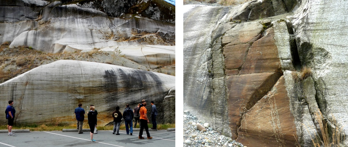
glacial groove (Chapter 16) a straight line created on a rock surface by erosion by a rock fragment embedded in the base of glacial ice (larger and deeper than a glacial striation)
glacial striation (Chapter 16) a straight line created on a rock surface by erosion by a rock fragment embedded in the base of glacial ice (finer than a glacial groove – typically less than 1 centimetre wide)
glacier (Chapter 16) a long lasting (centuries or more) body of ice on land that moves under its own weight
glaciofluvial (Chapter 16) referring to sediments deposited from a stream that is derived from a glacier
glaciolacustrine (Chapter 16) referring to sediments deposited within a lake in a glacial environment
glaciomarine (Chapter 16) referring to sediments deposited within the ocean in a glacial environment
glaucophane (Chapter 7) a blue-coloured sodium-magnesium bearing amphibole mineral that forms during metamorphism at high pressures and relatively low pressures, typically within a subduction zone
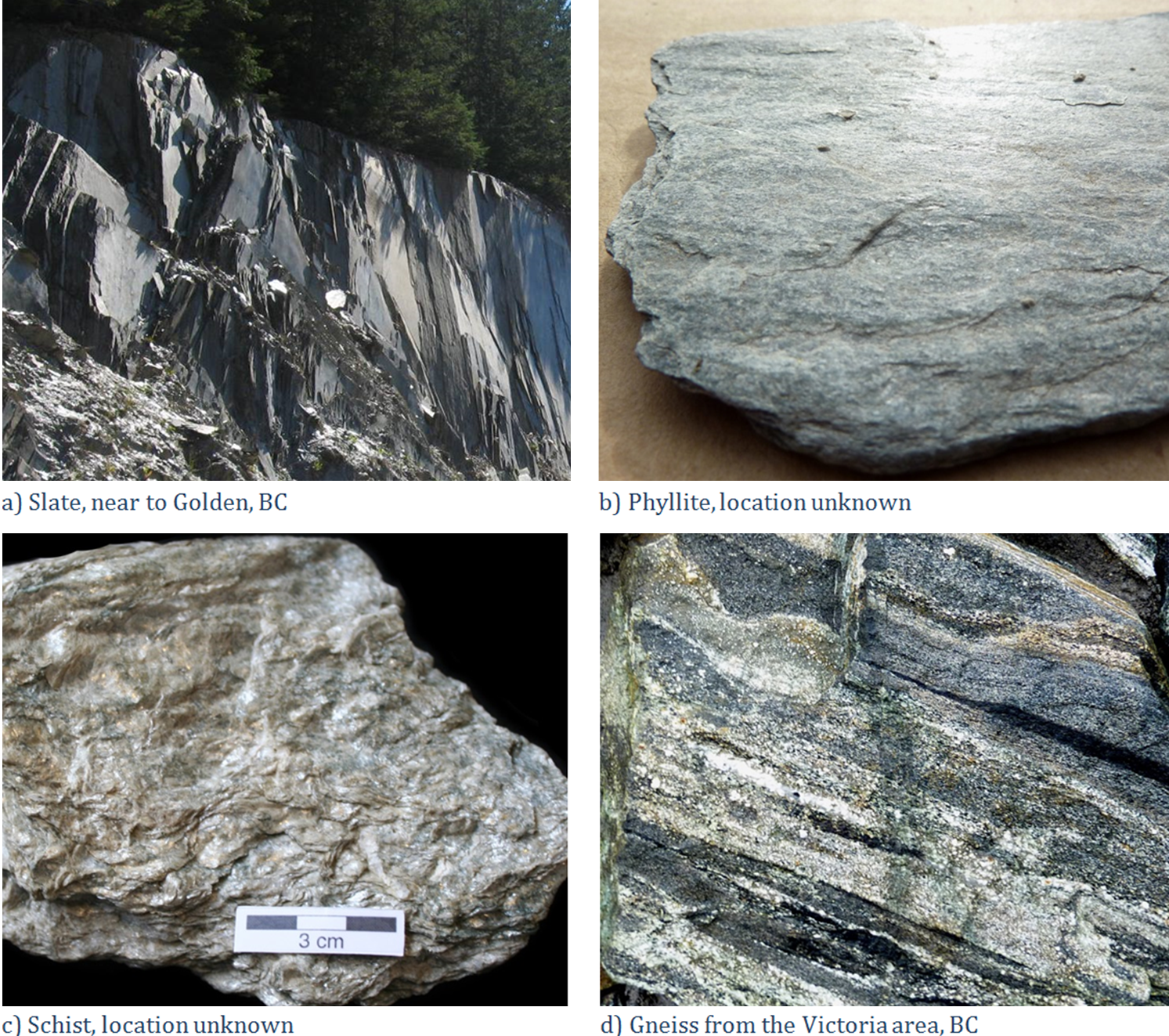
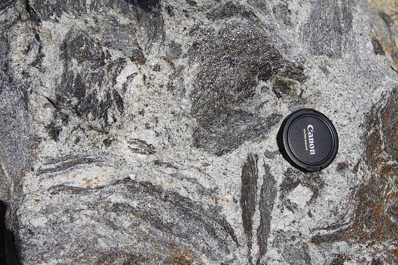
gneiss (Chapter 7) high-grade metamorphic rock in which the mineral components are separated into bands
graben (Chapter 12) a down-dropped fault block, bounded on either side by normal faults
grade (Chapter 7) in the context of a mineral deposit, the amount of a specific metal or mineral expressed as a proportion of the whole rock
graded bedding (Chapter 6) an individual sedimentary layer that shows a distinctive gradation in grain size (normal graded bedding is finer towards the top, reverse graded bedding is coarser towards the top)
gradient (Chapter 13) the slope of a stream bed over a specific distance, typically expressed in m per km
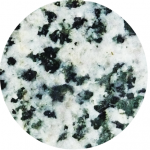
granite (Chapter 1) a felsic intrusive igneous rock
granule (Chapter 6) a sedimentary particle ranging in size from 2 to 4 millimetres in diameter
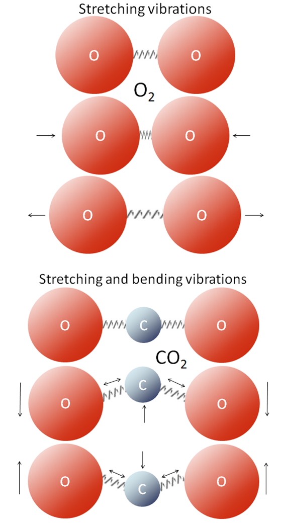
greenhouse gas (Chapter 22) a gaseous molecule with 3 or more atoms that is able to absorb infrared radiation
greenhouse effect (Chapter 22) in the context of climate, the ability of an atmosphere to absorb infrared radiation due to the presence of greenhouse gases
greenschist (Chapter 7) a foliated metamorphosed rock (typically derived from basalt) in which the green colouration is derived from either chlorite, epidote or green amphibole
greenstone (Chapter 7) a non-foliated metamorphosed rock (typically derived from basalt) in which the green colouration is derived from either chlorite, epidote or green amphibole
greywacke (Chapter 6) a sandstone with more than 15% silt and clay, and with a significant proportion of sand-sized rock fragments
groundwater (Chapter 13) water that lies beneath the surface of the ground
group (Chapter 6) a stratigraphically-continuous series of related formations
groyne (Chapter 17) a man-made structure extending from the shore built to deflect the energy of waves
gyre (Chapter 18) a closed circular ocean current
H
habit (Chapter 2) a characteristic crustal form or combination of forms of a mineral
habitable zone (Chapter 22) the region around a star that is considered to be suitable for a life-bearing planet
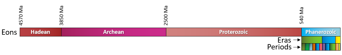
Hadean (Chapter 1) the first eon of Earth history, extending from 4.57 to 3.80 Ga
halide (Chapter 2) a mineral in which the anion is one of the halide elements (e.g., halite – NaCl or fluorite – CaF2)
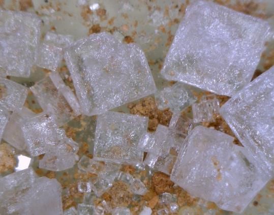
halite (Chapter 1) NaCl, a halide mineral also known as table salt
halogen (Chapter 2) an element in the second-last column of the periodic table that forms anions with a negative-1 charge
hanging valley (Chapter 16) a glacial valley created by a tributary glacier which does not erode as deeply as the main-valley glacier that it joins
hanging wall (Chapter 12) the upper surface of a non-vertical fault
headland (Chapter 17) a point extending out to sea
horn (Chapter 16) a peak that has been eroded on at least three sides by glaciers
hornfels (Chapter 7) a fine-grained metamorphic rock that is not foliated
horst (Chapter 12) an uplifted fault block, bounded on either side by normal faults
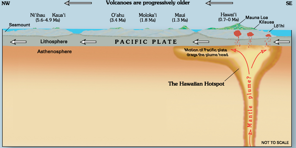
hot spot (Chapter 10) the surface area of volcanism and high heat flow above a mantle plume
hydrated mineral (Chapter 7) a mineral that includes either hydroxyl (OH) or water (H2O) in its chemical formula (e.g., gypsum CaSO4.2H2O)
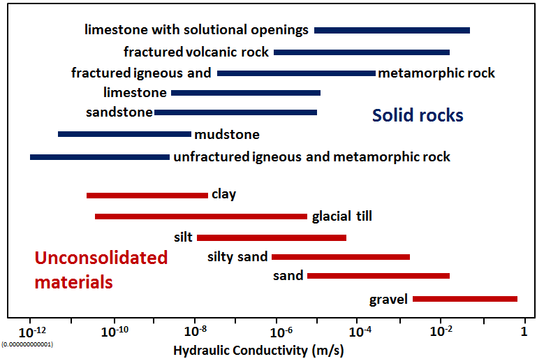
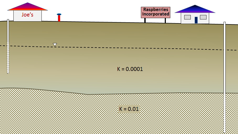
hydraulic conductivity (Chapter 14) an expression of the rate at which a liquid will flow through a porous medium, as determined by the permeability of the medium and the viscosity of the liquid
hydraulic fracturing (Chapter 20) fracturing rock by injecting water and chemicals down a well at very high pressure (equivalent to fracking)
hydrolysis (Chapter 5) a reaction between a mineral and water in which H+ ions are added to the mineral and a chemically equivalent amount of cations are released into solution
hydroxide (Chapter 2) the anion OH- or an mineral that includes that anion
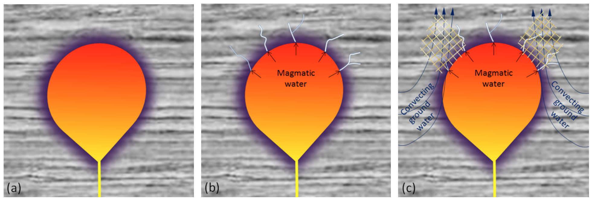
hydrothermal alteration (Chapter 7) chemical alteration of minerals by hot water solutions
hypocentre (Chapter 11) the actual point below surface at which an earthquake takes place (equivalent to focus)
I
ice giant (Chapter 22) a planet that is comprised mainly of gases heavier than hydrogen and helium, including oxygen, carbon, nitrogen, and sulfur (e.g., Uranus and Neptune)
igneous (Chapter 3) a rock formed from the cooling of magma
illite (Chapter 2) a clay mineral with a composition similar to that of muscovite mica
imbricate (Chapter 6) aligned and overlapping, like the tiles on a roof
index fossil (Chapter 8) a fossil with a distinctive appearance and a wide geographic range but from a relatively restricted time range, thus making it useful for dating a correlating rocks from different regions (the most useful index fossils are from organisms that lived for less than a million years)
inert (Chapter 2) in chemistry, an element that does not readily react with other elements (e.g., neon)
infiltration (Chapter 14) the recharge of groundwater from the downward percolation of surface water
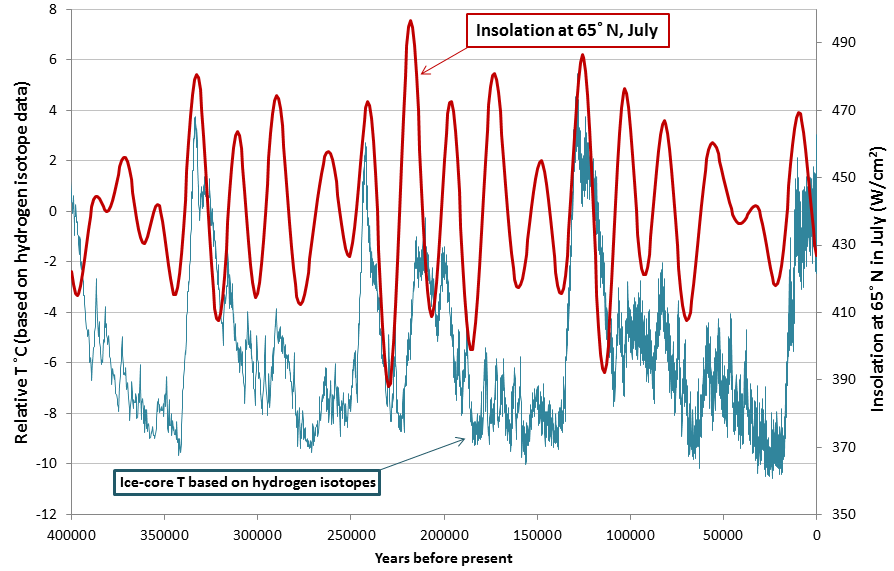
insolation (Chapter 19) a measure of the intensity of solar energy at a specific location or time (expressed in W/m2)
intensity (Chapter 11) in seismology, a qualitative measure of the amount of shaking at specific location, based on what was felt by observers, or the amount of damage done
Intergovernmental Panel on Climate Change (Chapter 19) (IPCC) an international body established in 1988 by the UN’s World Meteorological Organization and the UN Environment Program to prepare periodic reports on the status of global climate change and its mitigation
intrusive (Chapter 3) an igneous rock that has cooled slowly beneath the surface
ionic bond (Chapter 2) a bond in which electrons are transferred from one atom to another, thus forming ions
ion (Chapter 2) an atom that has either gained or lost electrons and has thus become charged (or a group of atoms that also has a charge – e.g., HCO3-)
isoclinal fold (Chapter 12) a tight fold in which the limbs are parallel to each other
isostasy (Chapter 9) the equilibrium between a block of crust floating on the underlying plastic mantle
isostatic sea level change (Chapter 17) the effect on relative sea level of a vertical adjustment of the crust resulting from a change in the mass of the crust (e.g., from losing or gaining ice)
isotope (Chapter 8) an form of an element that differs from other forms because it has a different number of neutrons (e.g., 16O has 8 protons and 8 neutrons while 18O has 8 protons and 10 neutrons)
J
joint (Chapter 12) a fracture in rock
Jovian planet (Chapter 22) a gas giant
K
ka (Chapter 1) (kilo annum) thousands of years before the present
kaolinite (Chapter 2) a clay mineral that does not have cations other than Al and Si
karst (Chapter 14) the solutional erosion of an area with soluble rock (typically limestone) to form depressions and caves
kettle (Chapter 16) a depression formed at the front of a large glacier when a stranded ice block that was surrounded by sediment eventually melts
kettle lake (Chapter 16) a lake that forms within a kettle
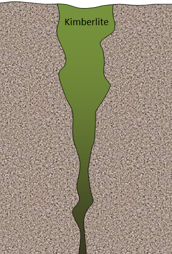
kimberlite (Chapter 4) an ultramafic volcanic rock that originates at significant depth (> 200 metres) in the mantle (some kimberlites include diamonds)
Kuiper belt (Chapter 22) a region of the Solar System beyond the orbit of Neptune that is populated by small objects and dwarf planets (including Pluto)
L
laccolith (Chapter 3) concordant intrusion in which the central part has formed an upward dome
lahar (Chapter 4) a mudflow or debris flow that is either caused by a volcanic eruption, or forms on the flank of a volcano as a result of flooding not related to an eruption
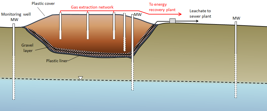
landfill gas (Chapter 14) gases produced within a landfill during the microbial breakdown of landfill components (most are dominated by carbon dioxide and methane)
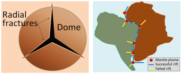
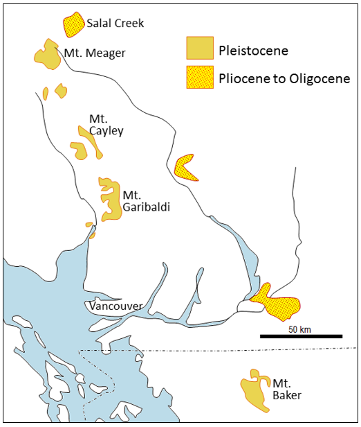
large igneous province (Chapter 4) a very large area of mafic volcanic rock produced by a massive eruption typically related to a mantle plume
lateral moraine (Chapter 16) a deposit of rocky material that forms along the margin of a valley or alpine glacier, mostly from the freeze-thaw release of material from the steep slopes above
lattice (Chapter 1) the regular and repeating three-dimensional structure of a mineral
Laurentide Ice Sheet (Chapter 16) the continental glacier that extended across central eastern North America during the Pleistocene, covering most of Canada and a significant part of the United States
lava levée (Chapter 4) a ridge that forms along the edge of a lava flow because the magma at the edge cools faster than that in the middle
lava tube (Chapter 4) a tube that forms as mafic lava flows along a channel and lava leveés build up on either side, eventually forming a roof (once a lava tube forms it insulates the flowing magma, allowing it to stay hot a liquid for longer and therefore flow much further)
leachate (Chapter 14) in the context of landfills, the liquid (rainwater) that passes through the waste and becomes contaminated with soluble components from the waste
levée (Chapter 13) on a stream, the ridge that naturally forms along the edge of the channel during flood events
level (Chapter 20) in mining, a horizontal mine opening
light year (Chapter 22) the distance that light can travel in one year (9.4607 x 10¹² km)
lignite (Chapter 20) a low-grade type of coal with less than 70% carbon
limbs (Chapter 12) the layers of rock on either side of a fold
limestone (Chapter 6) a sedimentary rock that is comprised mostly of calcite
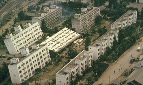
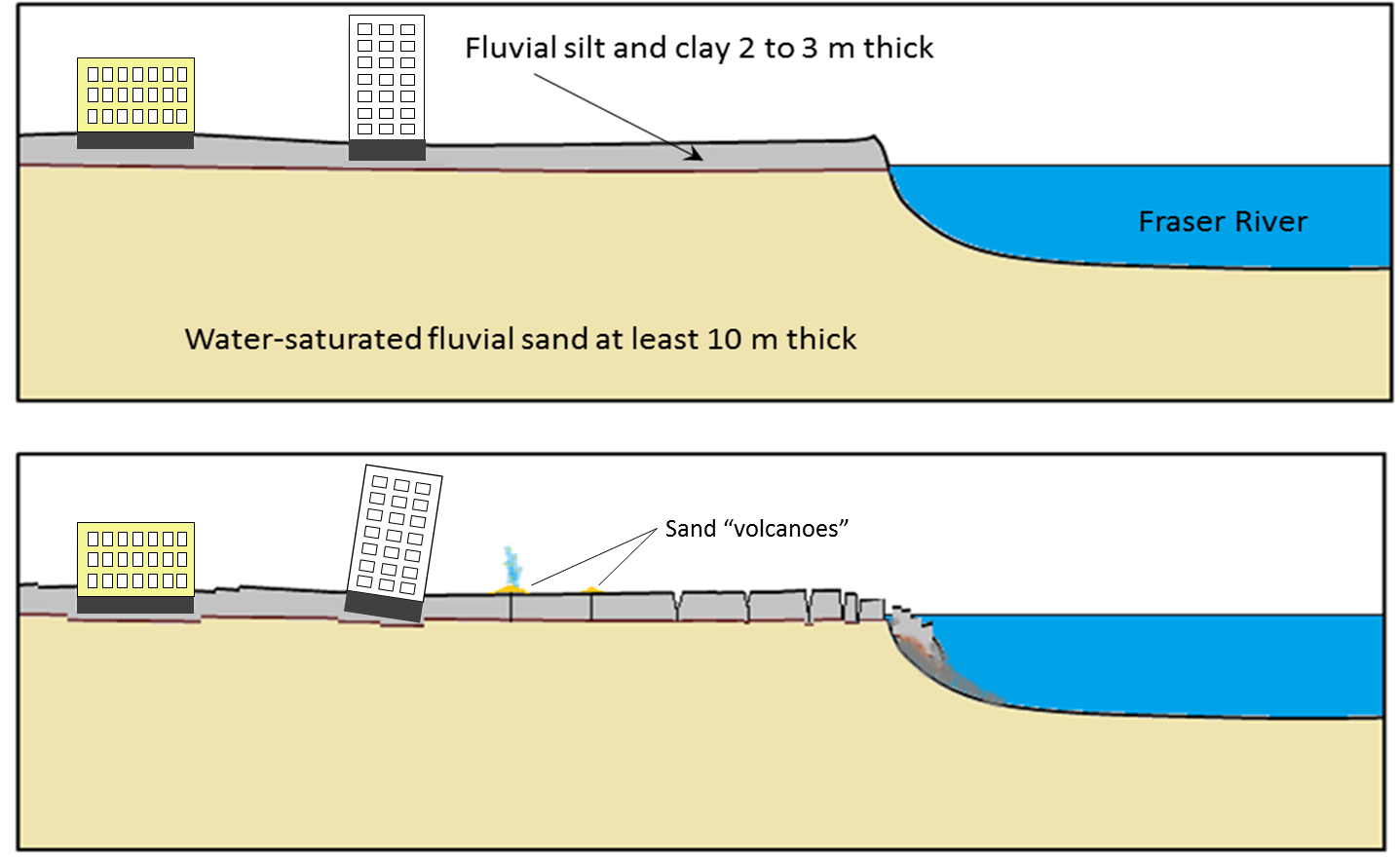
liquefaction (Chapter 11) the tendency for unconsolidated and water saturated sediments to lose strength during seismic shaking
lithic arenite (Chapter 6) an arenite in which there is more than 10% lithic clasts and in which there are more lithic clasts than feldspar clasts
lithic clasts (Chapter 6) fragments of rock (e.g., basalt) that are included in the sand-sized grains in sandstone, or in the larger grains in conglomerate
lithification (Chapter 6) the conversion of unconsolidated sediments into rock by compaction and cementation
lithosphere (Chapter 1) the rigid outer part of the Earth, including the crust and the mantle down to a depth of about 100 kilometres
lodgement till (Chapter 16) sediment that accumulates at the base of a glacier and typically has a wide range of grain sizes (including clay) and is well compacted
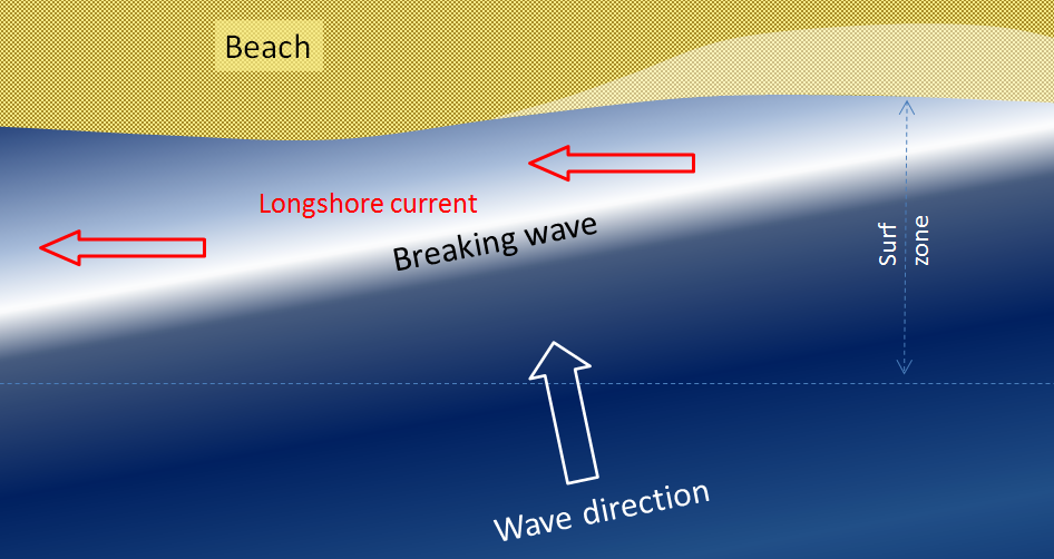
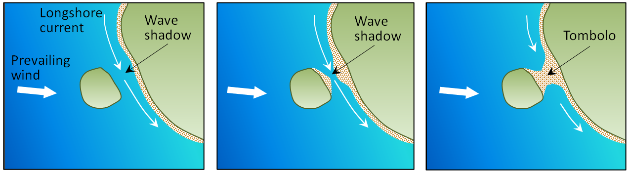
longshore current (Chapter 17) the movement of water along a shoreline produced by the approach of waves at an angle to the shore
longshore drift (Chapter 17) the movement of sediment along a shoreline resulting from a longshore current and also from the swash and backwash on a beach face
Love wave (Chapter 11) a surface seismic wave, with horizontal motion, that develops in relatively weak (e.g., unconsolidated) materials at surface
luvisol (Chapter 5) a cold climate forest soil formed in which clay has been removed from the A horizon and relocated into the B horizon
M
Ma (Chapter 1) (Mega annum) millions of years before the present
mafic (Chapter 3) silica poor (<45% SiO2) in the context of magma or igneous rock
magma (Chapter 1) molten rock typically dominated by silica
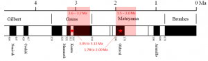
magnetic chronology (Chapter 8) the study of the timing of reversals of the Earth’s magnetic field, and the application of that understanding to dating geological materials
magnitude (Chapter 11) a measure of the amount of energy released by an earthquake
mantle (Chapter 1) the middle layer of the Earth, dominated by iron and magnesium rich silicate minerals and extending for about 2900 kilometres from the base of the crust to the top of the core
mantle plume (Chapter 3) a plume of hot rock (not magma) that rises through the mantle (either from the base or from part way up) and reaches the surface where it spreads out and also leads to hot-spot volcanism
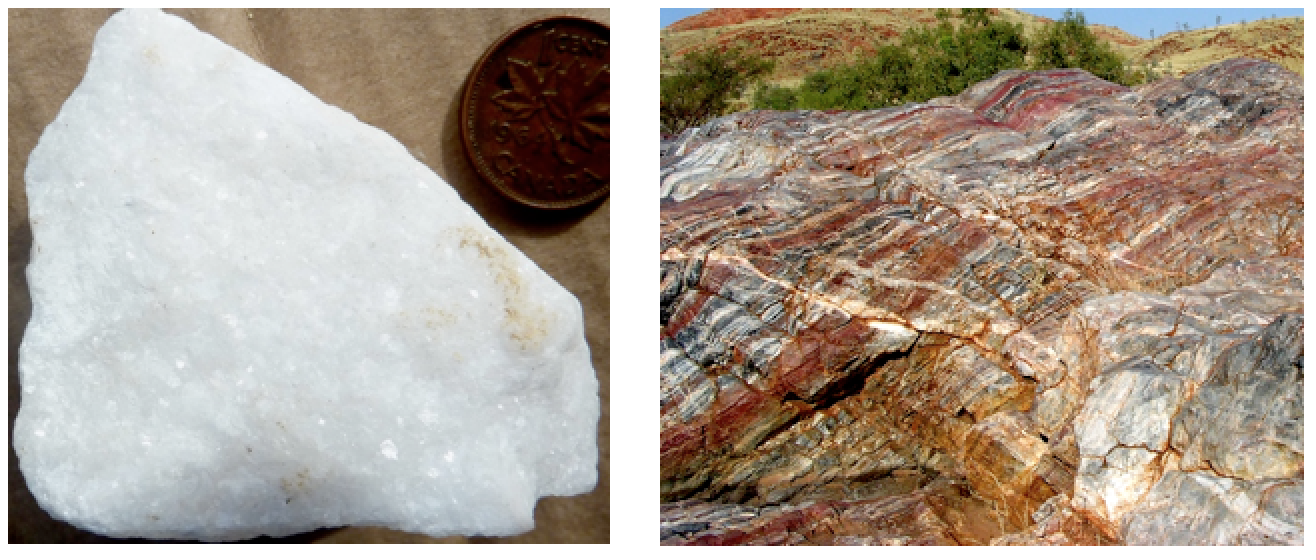
marble (Chapter 7) metamorphosed limestone (or dolostone) in which the calcite or dolomite has been recrystallized into larger crystals
mass wasting (Chapter 15) the mass failure, by gravity, of rock or unconsolidated material on a slope
meander cutoff (Chapter 13) the formation of a shorter stream channel across the narrow boundary between two meanders on a stream
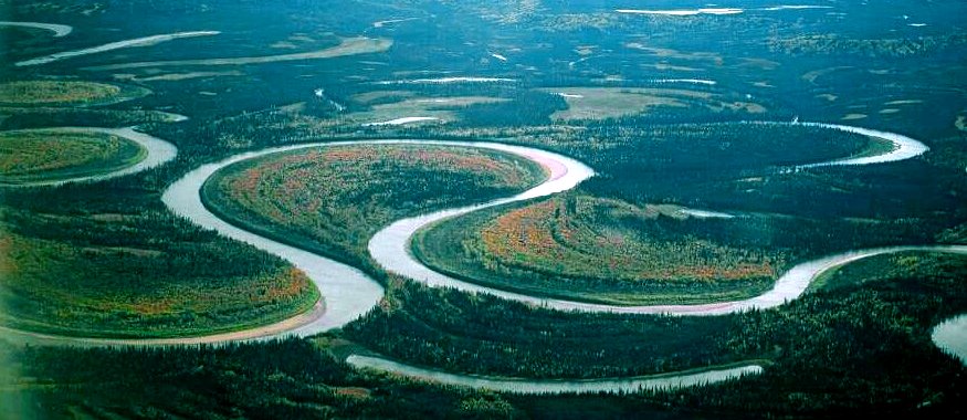
meandering (Chapter 13) the sinuous path taken by a stream within a wide flat flood plain
medial moraine (Chapter 16) a lateral moraine that has been shifted towards the centre of a valley glacier at a point where two glaciers meet
member (Chapter 6) a subdivision of a formation
mesopelagic zone (Chapter 18) the upper middle zone of the open ocean extending from a 200 to 1000 metre depth
metallic lustre (Chapter 2) the lustre of a mineral into which light does not penetrate but only reflects off of the surface
metallic bond (Chapter 2) a type of bond in which abundant electrons are easily shared amongst cations
metamorphism (Chapter 3) the transformation of a parent rock into a new rock as a result of heat and pressure that leads to the formation of new minerals, or recrystallization of existing minerals, without melting
metasomatism (Chapter 7) metamorphism facilitated by ion transfer through water
meteoroid (Chapter 22) a fragment of either stony or metallic debris in space
methane hydrate (Chapter 18) a combination of water ice and methane in which the methane is trapped inside “cages” in the ice
mica (Chapter 2) a sheet silicate mineral (e.g., biotite)
migmatite (Chapter 7) a rock that is a mixture of metamorphic and igneous rock, formed at very high grades of metamorphism when a part of the parent rock starts to melt
Milankovitch cycles (Chapter 19) millennial-scale variations in the orbital and rotational parameters of the Earth that have subtle effects on the Earth’s climate
Mohorovičić discontinuity (Chapter 9) the boundary between the crust and the mantle
moment magnitude (Chapter 11) a way of estimating earthquake magnitude based on the area of the rupture surface and the amount of displacement
monogenetic (Chapter 4) a volcano that forms in a single eruptive event
moraine lake (Chapter 16) a finger lake that forms within a glacial valley and is dammed by an end moraine
mud crack (Chapter 6) a dessication crack formed in mud that has accumulated in a small body of water that later dries up or drains
mudflow (Chapter 15) a mass-wasting event involving the flow of mud (sand, silt and clay) within a channel
mudrock (Chapter 6) an inclusive term for mudstone, shale and claystone
muscovite (Chapter 2) a potassium-bearing non-ferromagnesian mica
N
native element (Chapter 2) (also native element mineral) a mineral that consists of only one element (e.g., native gold)
nebula (Chapter 22) a cloud of interstellar dust and gases
negative feedback (Chapter 19) a process that results in a decrease in that process (in the context of climate change it is a process that reduces the change in climate, such as the enhanced growth of vegetation in response to an increase in atmospheric carbon dioxide)
neutron (Chapter 2) a sub-atomic particle with a mass of 1 and a charge of 0
nonconformity (Chapter 8) a geological boundary where non-sedimentary rock is overlain by sedimentary rock
non-ferromagnesian mineral (Chapter 2) a silicate mineral that does not contain iron or magnesium (e.g., feldsspar)
non-metallic lustre (Chapter 2) the lustre of a mineral into which light does penetrate
normal fault (Chapter 12) a non-vertical fault along which the hanging wall (upper surface) has moved down relative to the footwall
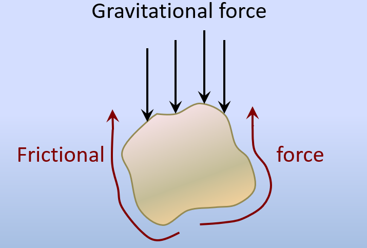
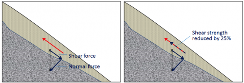
normal force (Chapter 15) the component of the gravitational force that acts directly into the slope
North Atlantic Deep Water (Chapter 18) deep Atlantic Ocean water that has descended in the far north of the basin in the area between Scandinavia and Greenland
nunatuk (Chapter 16) a rocky peak that extends above the ice level of a continental glacier
O
obliquity (Chapter 19) in the context of Milankovitch Cycles, the angle of the tilt of the Earth’s rotational axis with respect to the plane of its orbit around the Sun
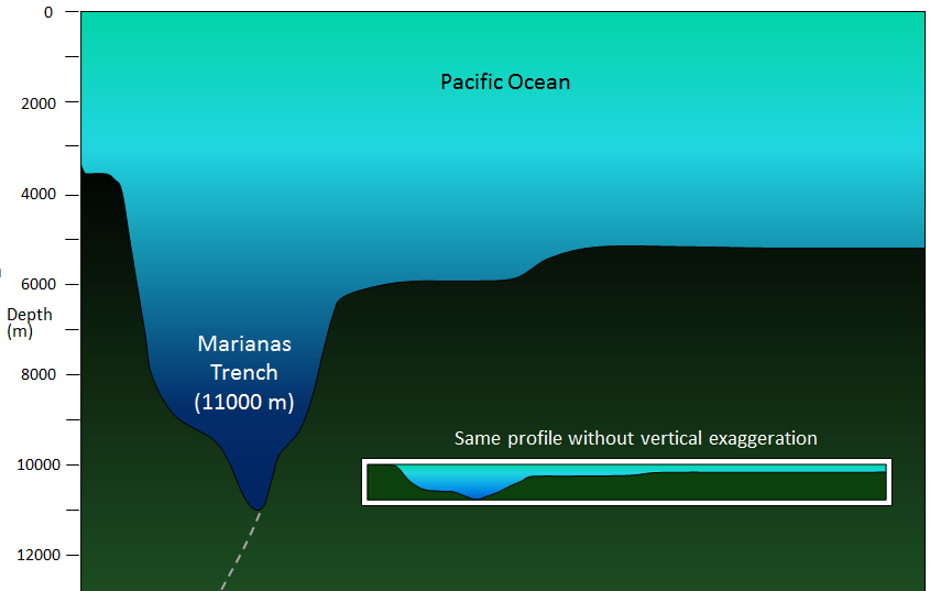
ocean plain (Chapter 18) the extremely flat surface of the deep ocean floor in areas unaffected by plate tectonic processes and volcanism
oil window (Chapter 20) the depth range, which is approximately 2000 to 4000 metres, within which the temperature is appropriate for the formation of oil from organic matter in sedimentary rock
ooid (Chapter 6) a small (approximately 1 millimetre) sphere of calcite formed in areas of tropical shallow marine water with strong currents
olivine (Chapter 2) a silicate mineral made up of isolated silica tetrahedra and with either iron or magnesium (or both) as the cations
Oort cloud (Chapter 22) a spherical cloud of icy objects extending from between about 5,000 and 500,000 astronomical units (Sun-Earth distances) from the Sun (thought to be the source area of comets)
open-pit mine (Chapter 20) a mine that is open to the surface
outcrop (Chapter 5) a surface exposure of rock that is part of the crust (bedrock)
outwash plain (Chapter 16) an extensive region of sand and gravel deposited by streams flowing out of a glacier (same as sandur)
overturned (Chapter 12) a geological feature that has been tilted to the point where it is upside down
oxbow (Chapter 13) a part of a stream meander that has become isolated from the rest of the stream as the result of a meander cutoff
oxidation (Chapter 5) the reaction between a mineral and oxygen
oxide (Chapter 2) a mineral in which the anion is oxygen (e.g., hematite Fe2O3)
P
pahoehoe (Chapter 4) a lava flow with a ropy surface texture formed when the surface cools and hardens while the lava beneath is still flowing
paleomagnetic (Chapter 10) past variations in the intensity and polarity of the Earth’s magnetic field
Pangea (Chapter 10) the supercontinent that existed between approximately 300 and 180 Ma
paraconformity (Chapter 8) an interruption representing a period of non-deposition, without tilting or erosion, in a sequence of sedimentary rocks
parasitic fold (Chapter 12) a fold within a fold
parent rock (Chapter 7) the rock that was already in existence when a process of metamorphism started
partial melting (Chapter 3) the process during which a only specific mineral components of a rock melt in response to changing conditions
parting (Chapter 6) a narrow gap between individual sedimentary layers
passive margin (Chapter 10) a boundary between a continent and an ocean at which there is no tectonic activity (e.g., the eastern edge of North America)
paternoster lake (Chapter 16) one of a series of rock basin lakes
pebble (Chapter 6) a sedimentary particle ranging in size from 2 to 64 millimetres (includes granule)
pelagic (Chapter 18) the part of a lake or the ocean that is not close to shore
permafrost (Chapter 19) ground that remains frozen for two or more years
permanentism (Chapter 10) the now discredited theory that the features on the Earth have not changed significantly over geological time
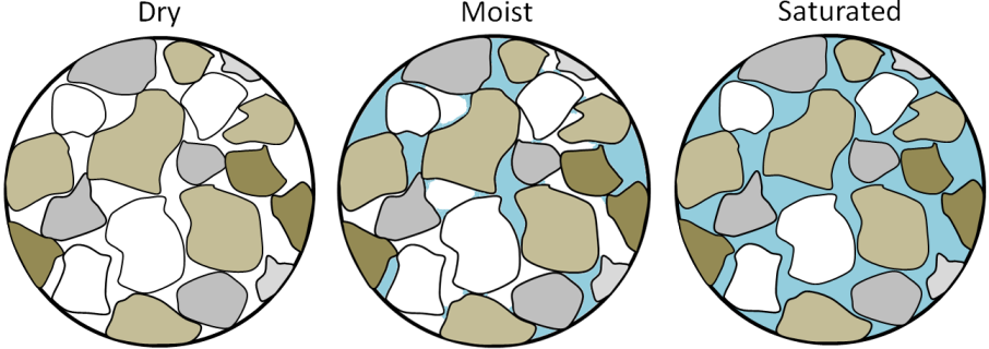
permeability (Chapter 14) an expression of the ease with which liquid will flow through a porous medium
phaneritic (Chapter 3) a rock texture in which the individual crystals or grains are visible to the naked eye
Phanerozoic (Chapter 1) the most resent eon of geological time, encompassing the Paleozoic, Mesozoic and Cenozoic
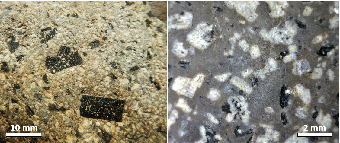
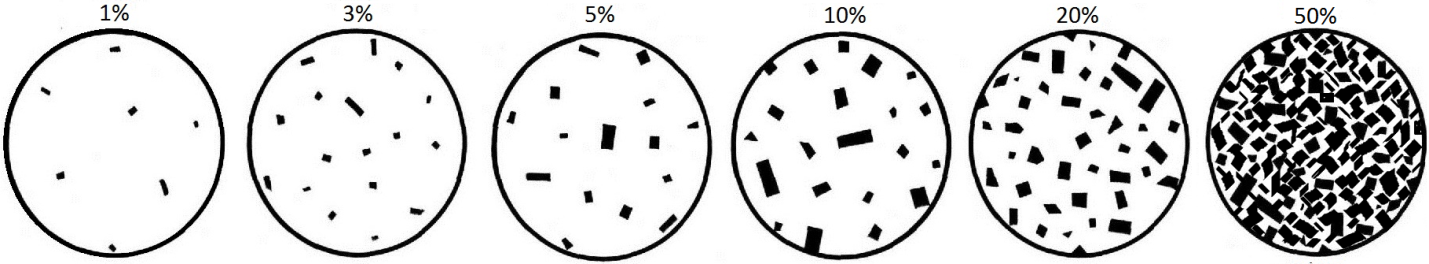
phenocryst (Chapter 3) a relatively large crystal within an igneous rock
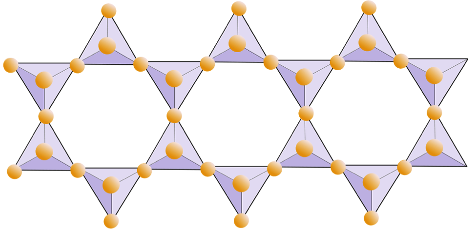
phyllosilicate (Chapter 2) a silicate mineral in which the silica tetrahedra are made up of sheets
phosphate (Chapter 2) a mineral in which the anion is PO43-
photic zone (Chapter 18) the upper 200 metres of the ocean or a lake, where, depending on the turbidity of the water, light can penetrate
phreatic eruption (Chapter 4) a steam-drive volcanic eruption that takes place when surface or near-surface water is heated by volcanic activity
phyllite (Chapter 7) a metamorphic rock with slaty cleavage and a sheen on the surface produced by aligned micas
pillow (Chapter 4) a pillow-shaped mass of volcanic rock (typically basalt) formed when magma erupts beneath the surface
pillow lava (Chapter 4) a volcanic rock (typically basalt) that is made up primarily of pillows
pipe (Chapter 3) a cylindrical body of igneous rock, typically resulting from a feeder conduit to a volcano
plate (Chapter 1) a region of the lithosphere that is considered to be moving across the surface of the Earth as a single unit
plate tectonics (Chapter 1) the concept that the Earth’s crust and upper mantle (lithosphere) is divided into a number of plates that move independently on the surface and interact with each other at their boundaries
plinian eruption (Chapter 4) a large volcanic eruption in which a column of hot tephra and gases rises many kilometres into the atmosphere
pluton (Chapter 3) a body of intrusive igneous rock
podsol (Chapter 55) a soil with well-developed horizons formed in temperate forested regions
podsolization (Chapter 5) the process of the formation of podsol
polar wandering path (Chapter 10) a path of varying magnetic pole positions defined by paleomagnetic data (in fact it is now understood that the continents have wandered, not the poles, so a more appropriate terms is “apparent polar wandering path”)
polymerize (Chapter 3) the formation of molecular chains within a fluid (e.g., a magma) that lead to an increase in the fluid’s viscosity
polymorphs (Chapter 7) two or more minerals with the same chemical formula but different crystal structures
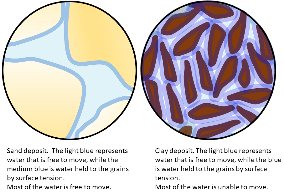
porosity (Chapter 14) the percentage of open pore space within a body of rock or sediment
porphyritic (Chapter 3) an igneous texture in which some of the crystals are distinctively larger than the rest
porphyry deposit (Chapter 20) a mineral deposit (of copper or molybdenum especially) in which part of the host rock is a porphyritic stock
positive feedback (Chapter 19) a process that results in an increase in that process (in the context of climate change it is a process that enhances the change in climate, such as the reduced reflectivity of the Earth’s surface when ice melts)
potassium feldspar (Chapter 2) feldspar with the formula KAlSi3O8
potentiometric surface (Chapter 14) the imaginary surface defined by the levels to which water would rise in a series of wells drilled into a confined aquifer
precession (Chapter 19) in the context of Milankovitch Cycles, the variation in the direction at which the Earth’s rotational axis is pointing
principle of cross-cutting relationships (Chapter 6) the principle that a body of rock that cuts across or through another body of rock is younger than that other body
principle of faunal succession (Chapter 6) the principle that life on Earth has evolved in an orderly way, and that we can expect to always find fossils of a specific type in rocks of a specific age
principle of inclusions (Chapter 6) the principle that inclusions within a body of rock must be older than the rock
principle of original horizontality (Chapter 6) the principle that sedimentary beds are originally deposited in horizontal layers
principle of superposition (Chapter 6) the principle that in a sequence of layered rocks that is not overturned or interrupted by faulting, the oldest will be at the bottom and the youngest at the top
proglacial (Chapter 16) referring to the area in front of a glacier
proton (Chapter 2) a sub-atomic particle with a mass of 1 and a charge of 1
protoplanetary disk (Chapter 22) a rotating cloud of gas and dust surrounding a young star
pumice (Chapter 4) a highly vesicular felsic volcanic rock (typically composed mostly of glass)
p-wave (Chapter 9) a seismic body wave that is characterized by deformation of the rock in the same direction that the wave is propagating (compressional vibration)
pyroclastic (Chapter 4) volcanic material formed during an explosive eruption
pyroclastic density current (Chapter 4) a body of hot pyroclastic rock and gases that is flowing rapidly down the flank of a volcano
pyroxene (Chapter 2) a single chain silicate mineral
Q
quartz (Chapter 2) a silicate mineral with the formula SiO2
quartz sandstone (Chapter 6) a sandstone in which more than 90% of the grains are quartz
quartzite (Chapter 7) a metamorphic rock formed from the contact or regional metamorphism of sandstone
R
radial (Chapter 13) a pattern of streams radiating out from a central point, typically an isolated mountain
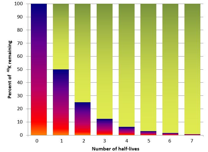
radioactivity (Chapter 9) the natural transformation of unstable isotopes into new elements
radiolaria (Chapter 18) microscopic (0.1 to 0.2 millimetres) marine protozoa that produce silica shells
Rayleigh wave (Chapter 11) a surface seismic wave, with vertical motion
recharge (Chapter 14) the transfer of surface water into the ground to become groundwater
recharge area (Chapter 14) an area of an aquifer where recharge is predominant over discharge
rectangular (Chapter 13) a drainage pattern in which tributaries typically flow at right angles to each other and meet at right angles
recumbent fold (Chapter 12) a fold that is overturned such that its limbs are close to horizontal
redshift (Chapter 22) the increase in wavelength of light resulting from the fact that the source of the light is moving away from the observer
reef (Chapter 17) a mound of carbonate formed in shallow tropical marine environments by corals, algae and a wide range of other organisms
regional metamorphism (Chapter 7) metamorphism caused by burial of the parent rock to depths greater than 5 kilometres (typically takes place beneath mountain ranges, and extends over areas of hundreds of km2)
remnant magnetism (Chapter 10) magnetism of a body of rock that formed at the time the rock formed and is consistent with the magnetic field orientation that existed at that time and place
reservoir rock (Chapter 20) rock into which petroleum has migrated and is now trapped
residual soil (Chapter 5) soil formed by weathering of the underlying rock or sediment
retrograde metamorphism (Chapter 7) metamorphism that takes place at a lower temperature than that at which the rock originally formed or was previously metamorphosed
reverse fault (Chapter 12) a non-vertical fault along which the hanging wall (upper surface) has moved up relative to the footwall
rhyolite (Chapter 3) a felsic volcanic rock
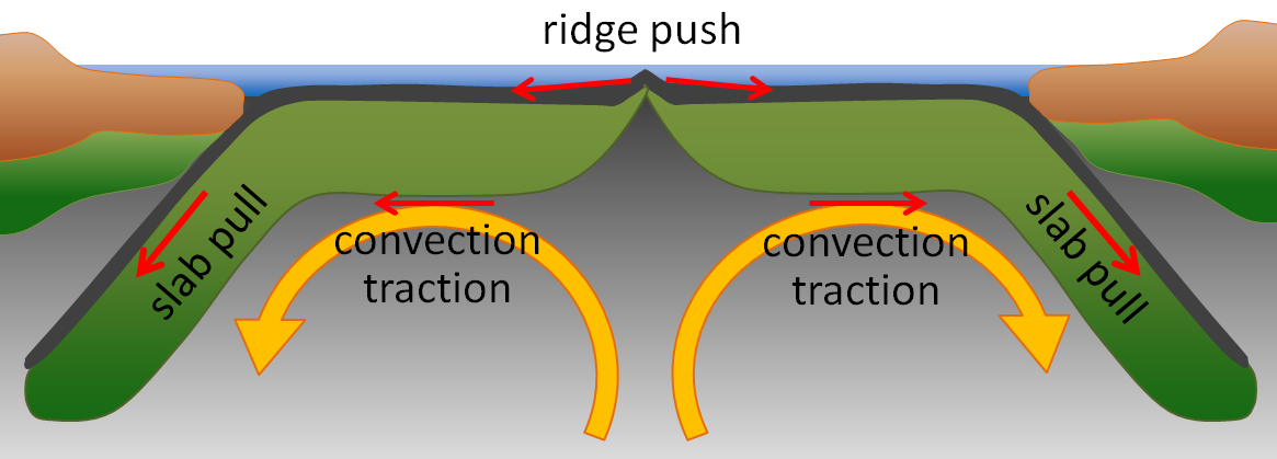
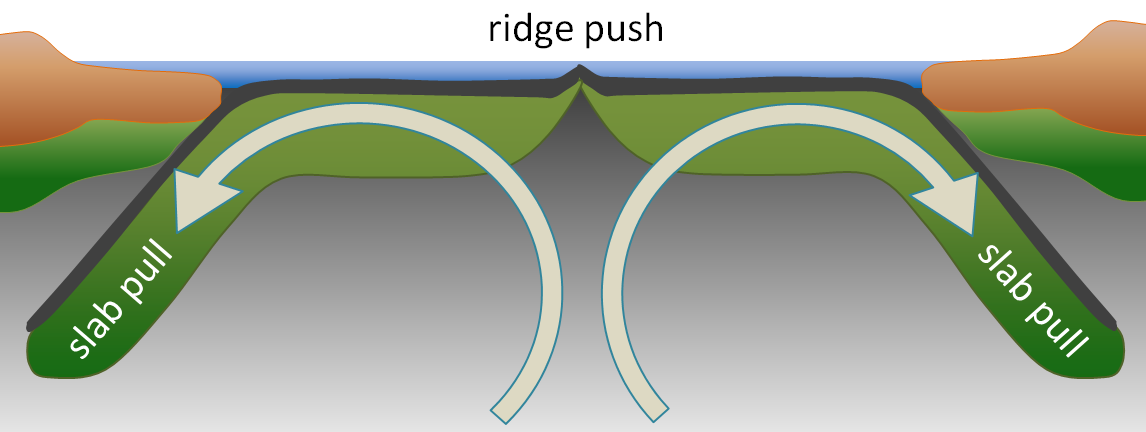
ridge push (Chapter 10) the concept that at least part of the mechanism of plate motion is the push of oceanic lithosphere down from a ridge area
rip current (Chapter 17) a strong flow of water outward from a beach
ripple (Chapter 6) on a series of small parallel ridges formed within sediment that has accumulated in moving water or wind
rip-rap (Chapter 17) angular rock fragments, typically boulder sized, used to armour slopes and shorelines against erosion
roche moutonée (Chapter 16) a product of glaciation in which a bedrock protrusion is eroded into a streamlined shape that has a broken or jagged leading (down-ice) edge
rock avalanche (Chapter 15) a rapid turbulent flow of broken bedrock fragments down a steep slope
rock basin lake (Chapter 16) a lake situated in a rock basin carved at the upper end of an alpine glacier
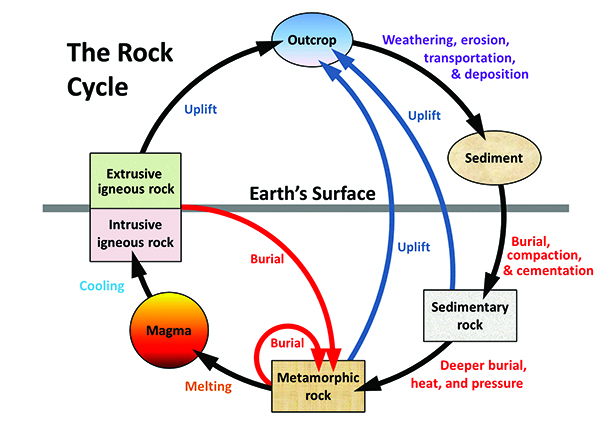
rock cycle (Chapter 3) the series of processes through which rocks are transformed from one type to another
rock fall (Chapter 15) the near-vertical fall or bouncing of rock released from a steep slope
rock slide (Chapter 15) the translational motion of an essentially intact body of rock down a slope (rock slides are typically slow, because once they start to move fast the rock body becomes fragmented and then flows as a rock avalanche)
runoff (Chapter 14) flow of water down a slope, either across the ground surface, or within a series of channels
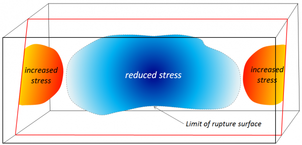
rupture (Chapter 11) breaking of rock subject to stress, typically resulting in an earthquake
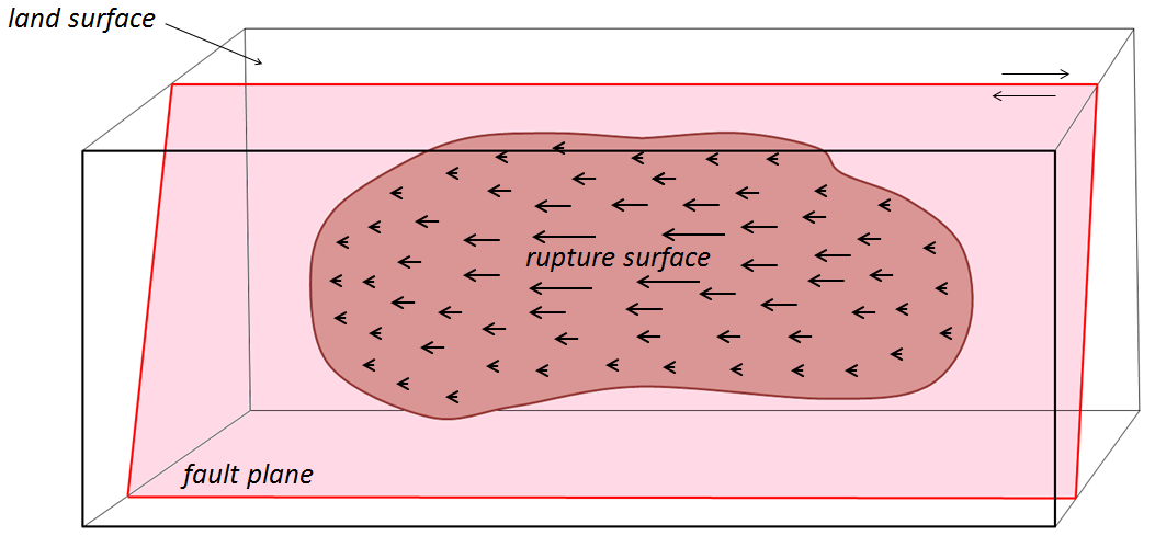
rupture surface (Chapter 11) the area over which rock rupture takes place during an earthquake
S
sackung (Chapter 15) an escarpment or trough at the top of a slow-moving rock slide (sackungen)
saltation (Chapter 13) the bouncing of particles along a stream bottom or desert floor
sand (Chapter 6) a mineral or rock fragment ranging in size from 1/16th to 2 millimetres
sandstone (Chapter 1) a rock that is primarily comprised of sand-sized particles
sandur (Chapter 16) an extensive region of sand and gravel deposited by streams flowing out of a glacier (same as outwash plain)
saturated zone (Chapter 14) the part of an aquifer, or any body of rock, that is saturated with water
schist (Chapter 1) a metamorphic rock with visible aligned mica crystals
sea cave (Chapter 17) a shallow cave formed on a rocky shore by wave erosion
sea cliff (Chapter 17) a coastal escarpment that is typically eroding inland as a result of wave action
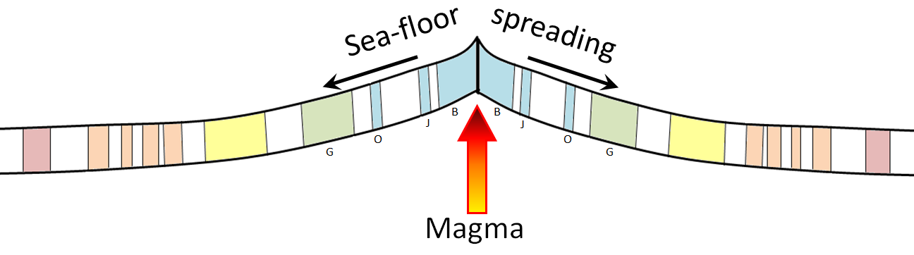
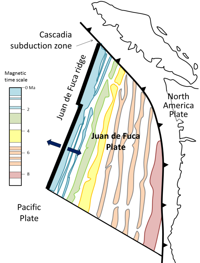
sea-floor spreading (Chapter 10) the formation of new oceanic crust by volcanism at a divergent plate boundary
sector collapse (Chapter 4) the sudden collapse of a significant part of the flank of a volcano
sedimentary rock (Chapter 3) rock that has formed by the lithification of sediments
sediments (Chapter 3) unconsolidated particles of mineral or rock
seismic (Chapter 11) pertaining to earthquakes
seismic moment (Chapter 11) a measurement of an earthquake’s energy based on longwave vibrations, or on the product of the fault area and displacement
seismic reflection sounding (Chapter 10) measurement of the properties of sediments based on detection of sounds generated at surface and reflected from layers beneath the surface
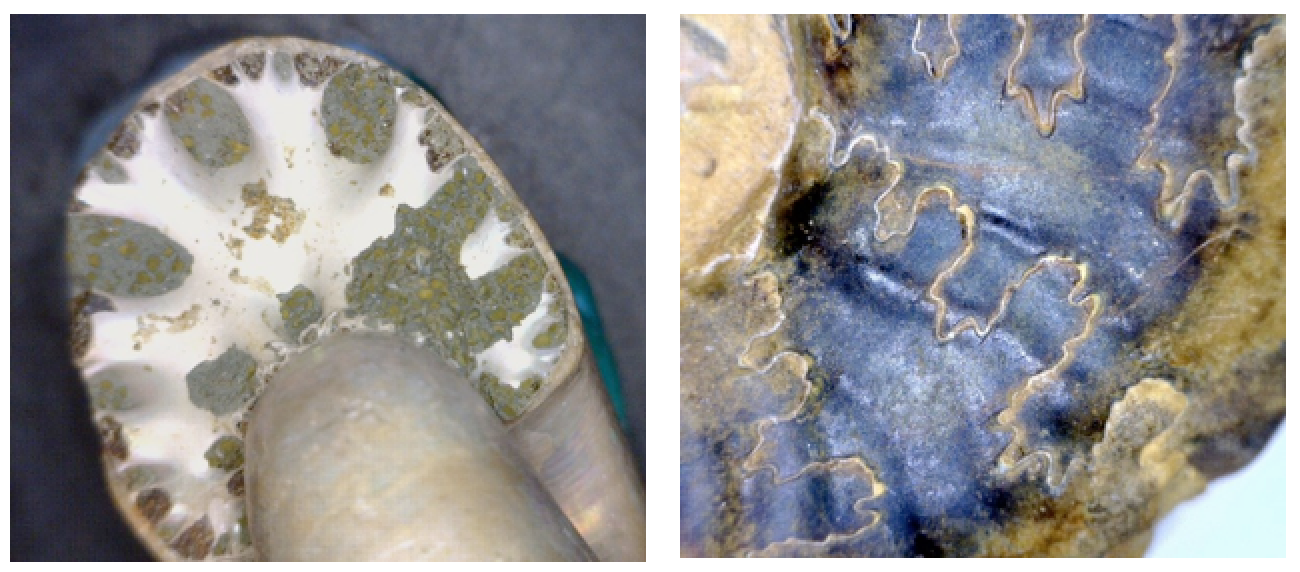
septae (Chapter 8) calcareous partitions between the successive living chambers in a cephalopod
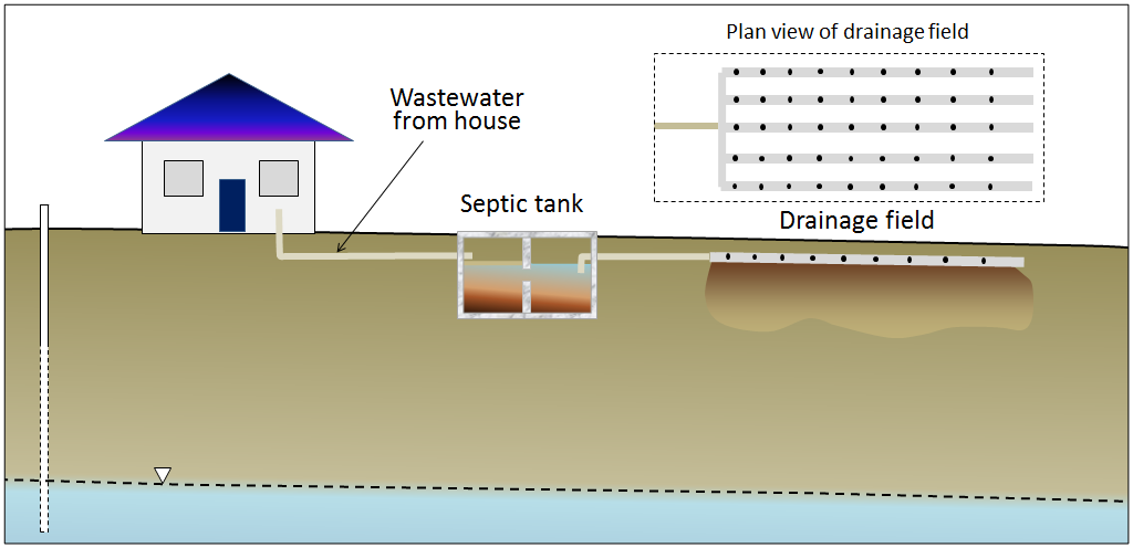
septic system (Chapter 14) a system constructed to facilitate the dispersion and detoxification of sewage (typically includes a septic tank and a drainage field)
shaft (Chapter 20) a vertical opening at a mine
shale (Chapter 6) a silt- and clay-rich rock that has evidence of layering
shear force (Chapter 15) the component of the gravitational force in the direction parallel to a slope
shear strength (Chapter 15) the strength of a body of rock or sediment that counteracts the shear force
shear stress (Chapter 12) the stress placed on a body of rock or sediment adjacent to a fault
sheeted dykes (Chapter 10) a series of near-vertical dykes formed in the vicinity of a spreading ridge when magma from depth flows into fractures formed by extensional forces
sheet silicate (Chapter 2) a silicate mineral in which the silica tetrahedra are combined within sheets
sheetwash (Chapter 5) overland flow of water, typically related to a heavy precipitation event
shield (Chapter 4) a region of ancient (typically Precambrian) crystalline rock (equivalent to a craton)
shield volcano (Chapter 4) a low-profile volcano formed primarily from eruptions of low-viscosity mafic magma
SIAL (sialic) (Chapter 10) referring to rock or magma in which silica and aluminum are the predominant components (generally equivalent to felsic)
silica (Chapter 2) a form of the mineral quartz (SiO2)
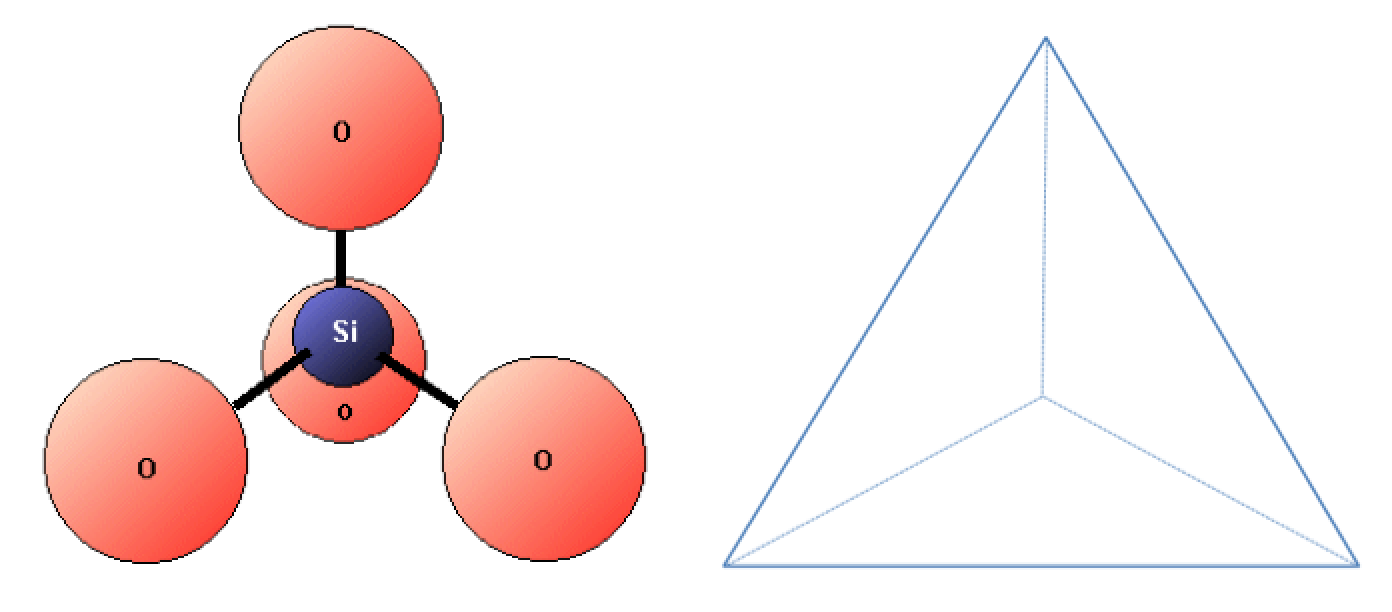
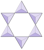
silica tetrahedron (Chapter 2) a combination of 1 silicon atom and 4 oxygen atoms that form a tetrahedron
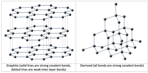
silicate (Chapter 1) a mineral that includes silica tetrahedra
silicon (Chapter 2) the 14th element
silicone (Chapter 2) resin or caulking made from silicon-oxygen chains and various organic molecules
sill (Chapter 3) an igneous intrusion that is parallel to existing layering in the country rock
silt (Chapter 6) sedimentary particles ranging is size from 1/256th to 1/16th of a millimetres
SIMA (simatic) (Chapter 10) referring to rock or magma in which silica, magnesium and iron are the predominant components (generally equivalent to mafic)
skarn (Chapter 7) the contact metamorphism (and metasomatism) of limestone
slab pull (Chapter 10) the concept that at least part of the mechanism of plate motion is the pull of oceanic lithosphere down into the mantle
slate (Chapter 7) a fine-grained metamorphic rock that splits easily into sheets
slaty cleavage (Chapter 7) the tendency for slate or phyllite to split into sheets (note that this is the only situation in this textbook where the term “cleavage” is applied to a rock as opposed to a mineral)
slide (Chapter 15) the downward movement of rock or sediment on a slope as an intact mass
slump (Chapter 15) a slide in which the nature of the motion is rotational (typically only develops in unconsolidated sediments)
smectite (Chapter 2) a fine-grained sheet silicate mineral that can accept water molecules into interlayer spaces, resulting is swelling
smelter (Chapter 20) a refinery at which minerals are processed to produce pure metals
snowline (Chapter 22) in astronomy the radius around a star at which represents the boundary between gases (or liquids) and solids
soil horizon (Chapter 5) a layer, within a well-developed soil, that is physically or chemically different from layers above or below
solar system (Chapter 22) a star and the planets surrounding it
solar wind (Chapter 22) a stream of ionized (charged) particles away from the Sun
solid solution (Chapter 2) the substitution of one element for another in a mineral (e.g., iron can be substituted for magnesium in the mineral olivine)
solifluction (Chapter 15) the flow of water saturated sediment or soil over a stronger and less permeable substrate
source rock (Chapter 20) the sedimentary rock from which petroleum originates prior to its migration into a reservoir rock
speleothem (Chapter 6) a solutionally-formed feature within a limestone cave (e.g., a stalactite)
spit (Chapter 17) a sand or coarser deposit extending from shore out into open water
spring (Chapter 14) the flow of groundwater onto the surface
stack (Chapter 17) a prominent rocky island that is a remnant of the erosion of a headland
stage (Chapter 13) the level of water in a stream
stalactite (Chapter 6) a cone-shaped speleothem that is suspended from the roof of a cave
stalagmite (Chapter 6) a cone-shaped speleothem that forms on the floor of a cave
step-pool (Chapter 13) a characteristic of stream flow in which water flows from one pool to another, typically on a stream with a steep gradient
stock (Chapter 3) an irregular pluton with n exposed area less than 100 km2
stoping (Chapter 3) the fracturing and incorporation of fragments of country rock as a magma body moves upward through the crust
strain (Chapter 12) the deformation of rock that is subjected to stress
streak (Chapter 2) the mark left on a porcelain plate when a mineral sample is ground to a powder by being rubbed across the plate (typically considered to provide a more reliable depiction of the colour than the whole sample)
stream (Chapter 13) any body of flowing water
stress (Chapter 12) a force applied to a rock
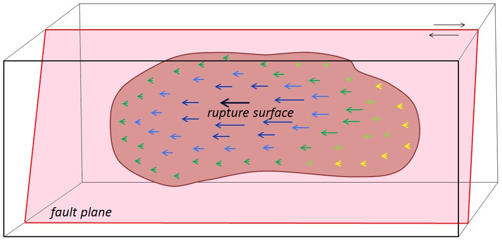
stress transfer (Chapter 11) the change in the pattern of stress on a region of rock as a result of an earthquake (typically stress is reduced in the area of a rupture zone, but is increased elsewhere in the vicinity)
strike (Chapter 12) the compass direction of a horizontal line on a sloped surface (e.g., bedding plane, fracture etc.)
strike-slip fault (Chapter 12) a fault that is characterized by motion that is close to horizontal and parallel to the strike direction of the fault
subaerial eruption (Chapter 4) a volcanic eruption that takes place on land
subaqueous eruption (Chapter 4) a volcanic eruption that takes place under water
subducted (Chapter 1) when part of a plate is forced beneath another plate along a subduction zone
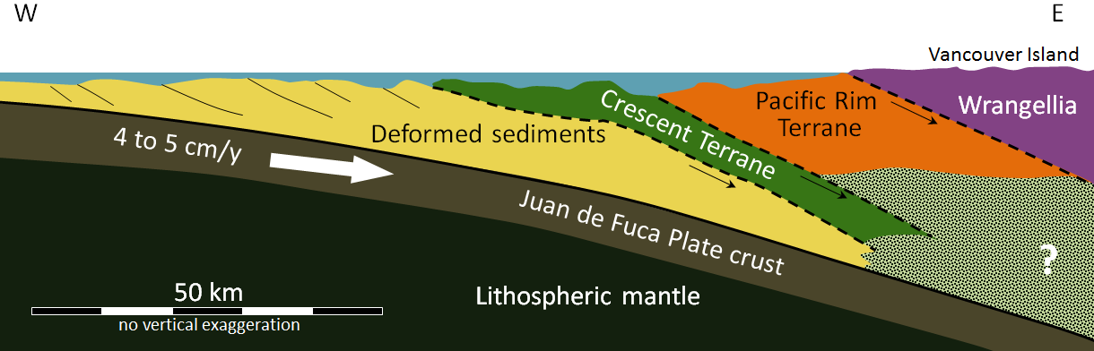
subduction zone (Chapter 10) the sloping region along which a tectonic plate descends into the mantle beneath another plate
subglacial (Chapter 16) beneath a glacier
sulphate (Chapter 2) a mineral in which the anion is SO42-
sulphide (Chapter 2) a mineral in which the anion is S2-
supergroup (Chapter 21) a stratigraphically-continuous series of related groups
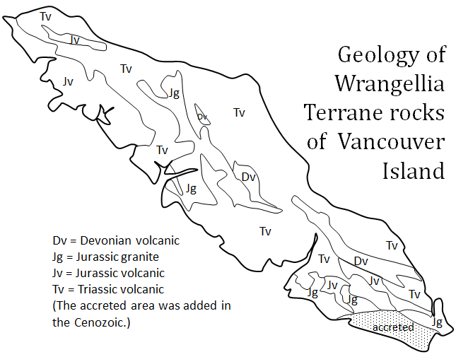
superterrane (Chapter 21) a number of terranes that are contiguous
supraglacial (Chapter 16) on the surface of a glacier
surf zone (Chapter 17) the near-shore zone where waves are breaking into surf
suture (Chapter 8) the line on the surface of a cephalopod that marks the boundary between a septum and the outer shell
swash (Chapter 17) the upward motion of a wave on a beach (typically takes place at the same angle that the waves are approaching the shore)
s-wave (Chapter 9) a seismic body wave that is characterized by deformation of the rock transverse to the direction that the wave is propagating
symmetrical (Chapter 12) a fold in which the limbs are at the same angle to the hinge
syncline (Chapter 12) a downward fold where the beds are known not to be overturned
synform (Chapter 12) a downward fold where it is not known if the beds are overturned
T
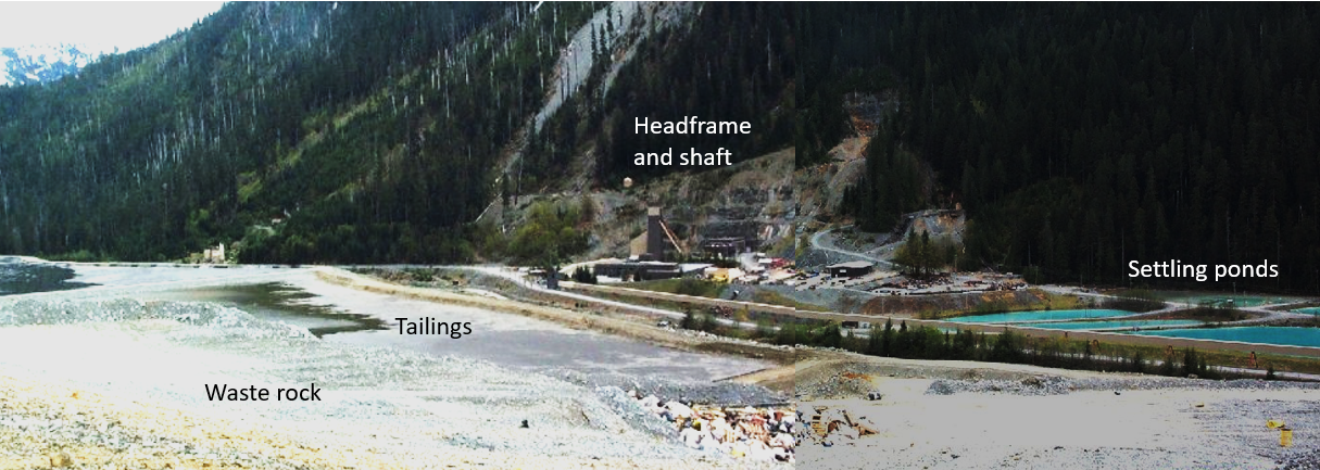
tailings (Chapter 20) the fine-grained waste rock from a plant used to concentrate ore minerals
talus slope (Chapter 15) a sloped deposit of angular rock fragments at the base of a rocky escarpment
tarn (Chapter 16) a lake within a rock basin
tectonic plate (Chapter 1) a region of the lithosphere that is considered to be moving across the surface of the Earth as a single unit
tectonic sea level change (Chapter 17) relative sea level change related to the vertical motion of a crustal block caused by tectonic processes
tephra (Chapter 4) fragments of volcanic rock (including volcanic ash) ejected during an explosive eruption
terminal moraine (Chapter 16) and end moraine that marks the farthest forward advance of a glacier
terrane (Chapter 7) a block of crust that has geological features that are distinctive from neighbouring regions, and is assumed to have been moved from elsewhere by tectonic processes
terrestrial planet (Chapter 22) a planet with a rocky mantle and crust and metallic core (e.g., Earth)
terrigenous (Chapter 18) referring to sedimentary particles that originated on a continent
test (Chapter 6) the shell-like hard parts (either silica or carbonate) of small organisms such as radiolarian and foraminifera
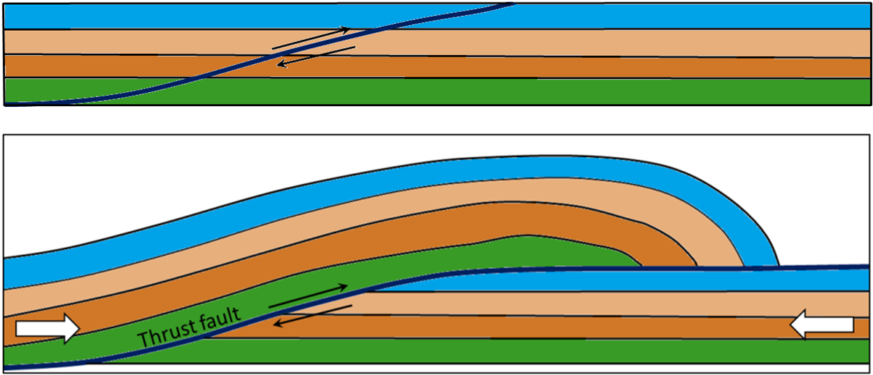
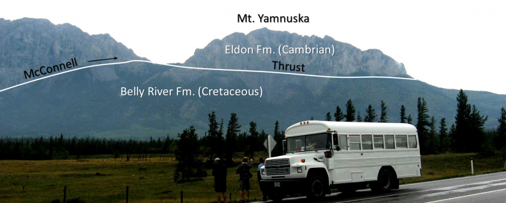
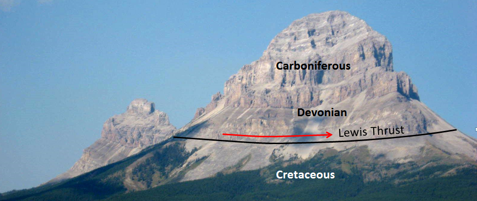
thrust fault (Chapter 11) a low angle reverse fault
till (Chapter 16) unsorted sediment transported and deposited by glacial ice
tiltmeter (Chapter 4) a sensitive instrument used to monitor subtle changes in the tilt of the land, particularly in studies of active volcanoes
tombolo (Chapter 17) a sand or coarser deposit connecting an island or rocky prominence to a larger body of land
traction (Chapter 13) a force that contributes to the movement of particles situated on a stream bed or desert floor
transform fault (Chapter 10) a boundary between two plates that are moving horizontally with respect to each other
travertine (Chapter 6) a deposit of calcium carbonate that forms at springs, hot springs or within limestone caves
trellis (Chapter 13) a drainage pattern in which tributaries typically flow parallel to one other but meet at right angles
trigger (Chapter 15) an event, such as an earthquake or a heavy rainfall, that triggers the onset of a mass wasting event
trough (Chapter 17) the lowest point of a wave
truncated spur (Chapter 16) the steep end of a ridge or arête that has been eroded by a main-valley glacier
tsunami (Chapter 11) a long-wavelength wave produced by the vertical motion of the floor of the ocean or a large lake, typically related either to an earthquake or a sub-marine mass wasting event
tufa (Chapter 6) a form of travertine that is especially porous as it forms around existing vegetative material.
tuya (Chapter 4) a flat-topped volcanic hill or mountain that formed when an eruption took place beneath a glacier and the melting led to the formation of a lake that then resulted in the wave-erosion of the top of the volcano
U
unconfined aquifer (Chapter 14) an aquifer that is not overlain by a confining layer
unconformity (Chapter 8) a geological boundary at the base of a sedimentary layer
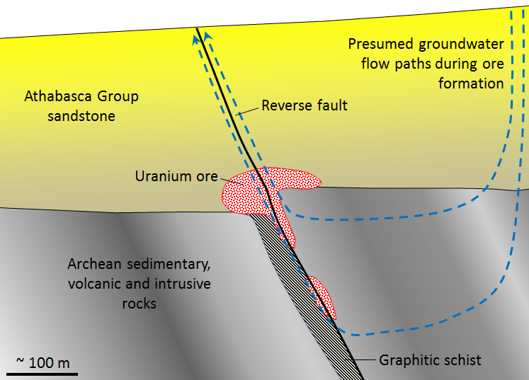
unconformity-type uranium deposit (Chapter 20) a uranium deposit that has formed at a nonconformity between sandstone and older rock
uncompressed density (Chapter 22) the density of planetary material that it would have it was not compressed by the planets gravitational force
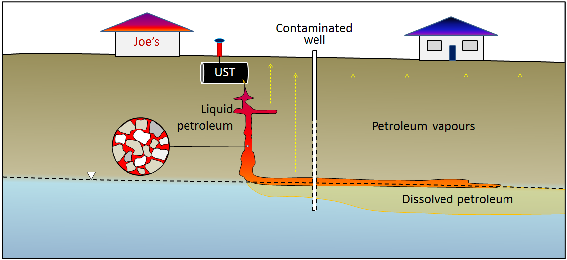
underground storage tank (Chapter 14) (UST) an underground tank for storing liquids, most commonly for liquid fuel
unsaturated zone (Chapter 14) the rock or sediment above the water table
U-shaped valley (Chapter 16) a relatively straight valley with a flat bottom and steep sides that has been carved by a valley glacier
V
valley glacier (Chapter 16) a glacier formed in a mountainous region and confined to a valley (same as alpine glacier)
varve (Chapter 16) a recognizable layer within sediments that represents a single year of deposition
vesicular (Chapter 3) an igneous texture characterized by holes left by gas bubbles
volcanic glass (Chapter 2) magma that has cooled within minutes, not allowing time for the formation of crystals
volcanic-hosted massive sulphide (Chapter 20) a mineral deposit hosted by volcanic rocks and including zones where most of the rock is made up of sulphide minerals (including ore minerals and pyrite)
W
wacke (Chapter 6) a sandstone with more than 15% clay and silt
water table (Chapter 14) the upper surface of the saturated zone in an unconfined aquifer
wave base (Chapter 17) the depth of water that is affected by the sub-surface orbital motion of wave action (approximately one-half of the wavelength)
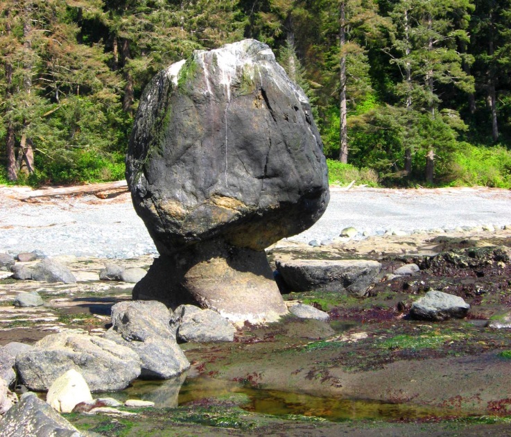
wave-cut platform (Chapter 17) a nearly-horizontal bench of rock eroded by waves within the surf zone (equivalent to wave-cut terrace)
wavelength (Chapter 17) the distance between the crests of two waves
weathering (Chapter 5) a range of processes taking place in the surface environment, through which solid rock is transformed into sediment and ions in solution
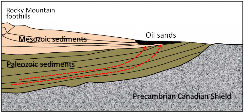
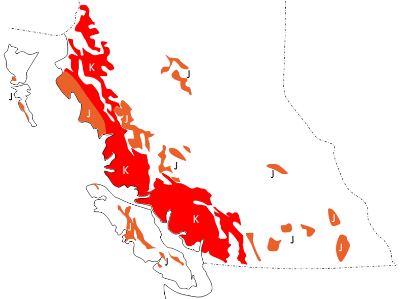
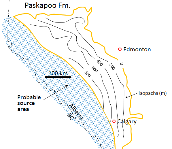
Western Canada Sedimentary Basin (Chapter 21) a large basin in the western interior of Canada, east of the Rocky Mountains, extending from the northern United States to the Northwest Territories
Wisconsin Glaciation (Chapter 16) the most recent advance of the Pleistocene glaciations, extending from 85 to 11 ka
X
xenolith (Chapter 3) a fragment of country incorporated into igneous rock, commonly as a result of stoping
Y
youthful stream (Chapter 13) a stream that is actively down-cutting its valley in an area that has recently been uplifted
Z
zone of ablation (Chapter 16) the part of a glacier, below the equilibrium line, where there is net loss of ice mass due to melting and calving
zone of accumulation (Chapter 16) the part of a glacier, above the equilibrium line, where there is net gain of ice mass because not all of the snow that falls each winter is able to melt during the following summer


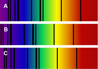

![Spectra for the sun and two galaxies. [KP]](https://opentextbc.ca/physicalgeology2ed/wp-content/uploads/sites/298/2019/08/spectra.png)
![Relative ages: 2: oldest: 3: middle, 1: youngest [SE]](https://opentextbc.ca/physicalgeology2ed/wp-content/uploads/sites/298/2019/08/ex8-1-300x269-1.png)

![Isotopic dating [SE]](https://opentextbc.ca/physicalgeology2ed/wp-content/uploads/sites/298/2019/08/ex8-3-300x182-1.png)
![Pangea [SE]](https://opentextbc.ca/physicalgeology2ed/wp-content/uploads/sites/298/2019/08/ex10-1-227x300-1.png)
![Pacific Plate rates of motion [SE]](https://opentextbc.ca/physicalgeology2ed/wp-content/uploads/sites/298/2019/08/ex10-2-274x300-1.png)
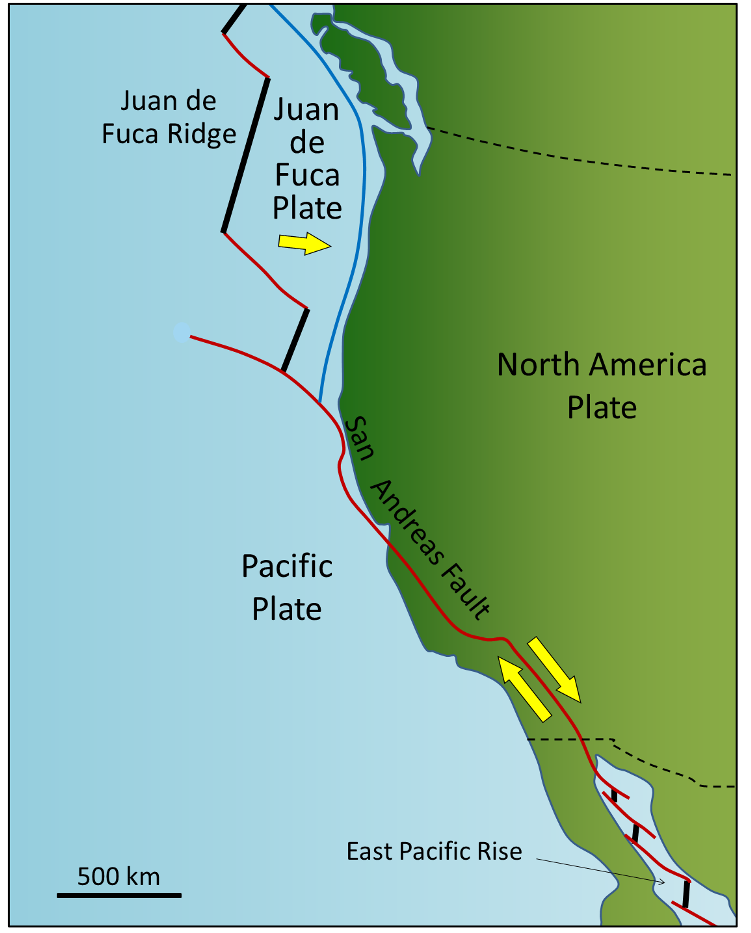
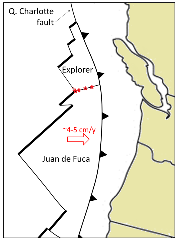
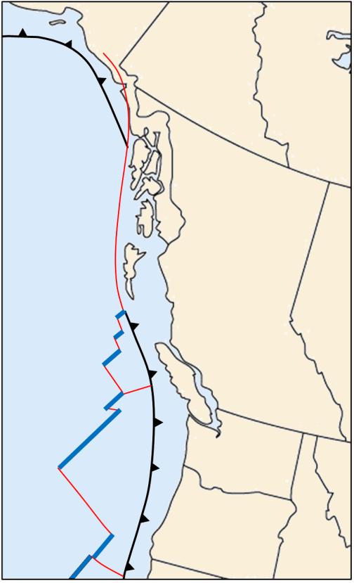
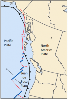
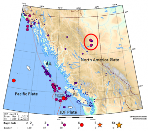
![Juan de Fuca and Explorer Plates [SE]](https://opentextbc.ca/physicalgeology2ed/wp-content/uploads/sites/298/2019/08/ex10-4-280x300-1.png)
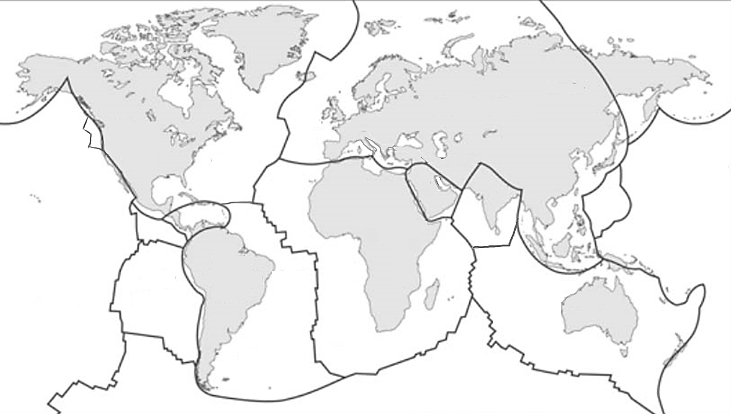
![The extents of the Earth's major plates [SE]](https://opentextbc.ca/physicalgeology2ed/wp-content/uploads/sites/298/2019/08/ex10-5-300x170-1.png)
![[SE]](https://opentextbc.ca/physicalgeology2ed/wp-content/uploads/sites/298/2019/08/ex13-3-300x205-1.png)
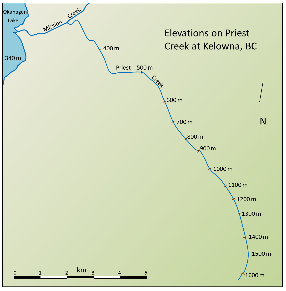
![Gradients of Priest Creek [SE]](https://opentextbc.ca/physicalgeology2ed/wp-content/uploads/sites/298/2019/08/ex13-4-300x300-1.png)
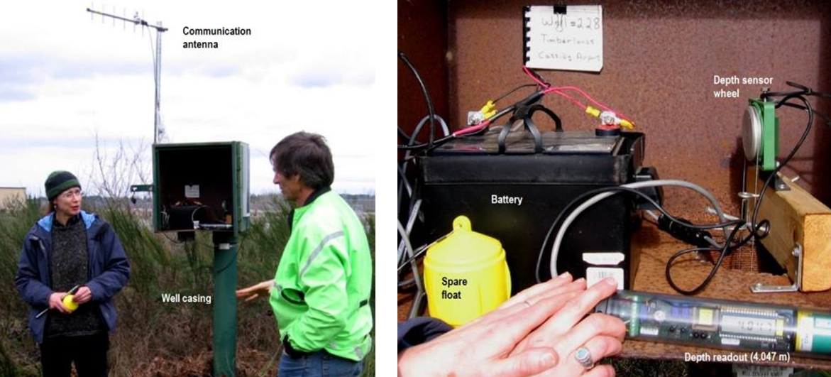
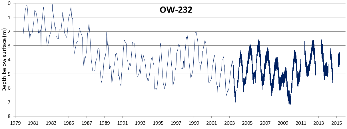
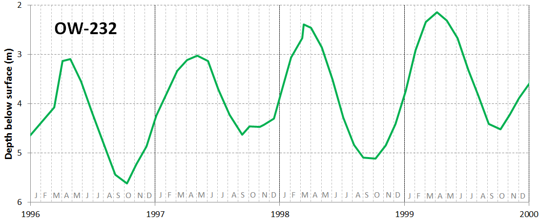
![[BC Ministry of the Environment at http://www.env.gov.bc.ca/wsd/data_searches/obswell/map/]](https://opentextbc.ca/physicalgeology2ed/wp-content/uploads/sites/298/2019/08/ex14-3-300x251-1.png)
![Implications of pumping from wells B and C and injecting into well A [SE]](https://opentextbc.ca/physicalgeology2ed/wp-content/uploads/sites/298/2019/08/ex14-6-300x129.png)
![[SE]](https://opentextbc.ca/physicalgeology2ed/wp-content/uploads/sites/298/2019/08/ex15-2-300x261.png)
![[SE]](https://opentextbc.ca/physicalgeology2ed/wp-content/uploads/sites/298/2019/08/ex16-1-300x178.png)
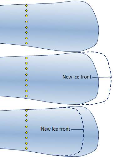
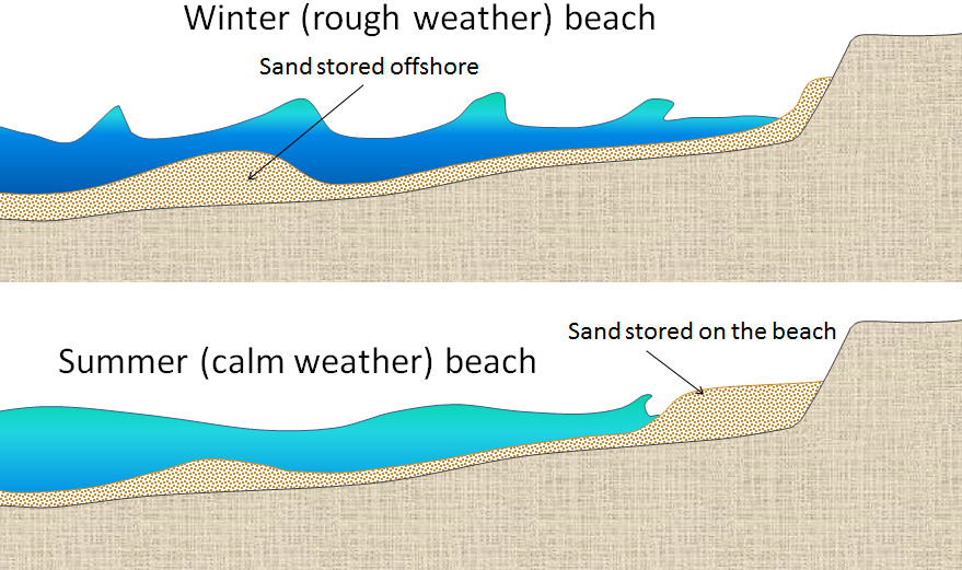
![Glacial advance (top) and retreat (bottom) [SE]](https://opentextbc.ca/physicalgeology2ed/wp-content/uploads/sites/298/2019/08/ex16-2-300x150.png)
![[SE after http://en.wikipedia.org/wiki/Mount_Assiniboine#/media/File:Mount_Assiniboine_Sunburst_Lake.jpg]](https://opentextbc.ca/physicalgeology2ed/wp-content/uploads/sites/298/2019/08/ex16-3-300x185.png)
![[SE]](https://opentextbc.ca/physicalgeology2ed/wp-content/uploads/sites/298/2019/08/ex17-2-300x144.png)
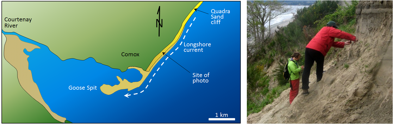
![Possible locations of coastal deposits [SE]](https://opentextbc.ca/physicalgeology2ed/wp-content/uploads/sites/298/2019/08/ex17-3-300x201.png)
![[SE]](https://opentextbc.ca/physicalgeology2ed/wp-content/uploads/sites/298/2019/08/ex17-5-300x124.png)
![[SE]](https://opentextbc.ca/physicalgeology2ed/wp-content/uploads/sites/298/2019/08/ex18-2-228x300.png)
![[SE]](https://opentextbc.ca/physicalgeology2ed/wp-content/uploads/sites/298/2019/08/ex18-3-300x96.png)
![[SE using climate data from Environment Canada, and ENSO data from: http://www.esrl.noaa.gov/psd/enso/mei/table.html]](https://opentextbc.ca/physicalgeology2ed/wp-content/uploads/sites/298/2019/08/ex19-4-300x153.png)
![[SE after USGS at: http://walrus.wr.usgs.gov/infobank/programs/html/definition/seis.html]](https://opentextbc.ca/physicalgeology2ed/wp-content/uploads/sites/298/2019/08/ex20-4-300x167.png)
![[SE after Geological Survey of Canada]](https://opentextbc.ca/physicalgeology2ed/wp-content/uploads/sites/298/2019/08/ex21-1-300x233.png)
![[SE]](https://opentextbc.ca/physicalgeology2ed/wp-content/uploads/sites/298/2019/08/ex21-3-300x229.png)
#/media/File:Hawaii_hotspot.jpg)
.jpg)
.jpg)
.jpg)