Main Body
Chapter 6. F-Test and One-Way ANOVA
F-distribution
Years ago, statisticians discovered that when pairs of samples are taken from a normal population, the ratios of the variances of the samples in each pair will always follow the same distribution. Not surprisingly, over the intervening years, statisticians have found that the ratio of sample variances collected in a number of different ways follow this same distribution, the F-distribution. Because we know that sampling distributions of the ratio of variances follow a known distribution, we can conduct hypothesis tests using the ratio of variances.
The F-statistic is simply:
[latex]F = s^2_1 / s^2_2[/latex]
where s12 is the variance of sample 1. Remember that the sample variance is:
[latex]s^2 = \sum(x - \overline{x})^2 / (n-1)[/latex]
Think about the shape that the F-distribution will have. If s12 and s22 come from samples from the same population, then if many pairs of samples were taken and F-scores computed, most of those F-scores would be close to one. All of the F-scores will be positive since variances are always positive — the numerator in the formula is the sum of squares, so it will be positive, the denominator is the sample size minus one, which will also be positive. Thinking about ratios requires some care. If s12 is a lot larger than s22, F can be quite large. It is equally possible for s22 to be a lot larger than s12, and then F would be very close to zero. Since F goes from zero to very large, with most of the values around one, it is obviously not symmetric; there is a long tail to the right, and a steep descent to zero on the left.
There are two uses of the F-distribution that will be discussed in this chapter. The first is a very simple test to see if two samples come from populations with the same variance. The second is one-way analysis of variance (ANOVA), which uses the F-distribution to test to see if three or more samples come from populations with the same mean.
A simple test: Do these two samples come from populations with the same variance?
Because the F-distribution is generated by drawing two samples from the same normal population, it can be used to test the hypothesis that two samples come from populations with the same variance. You would have two samples (one of size n1 and one of size n2) and the sample variance from each. Obviously, if the two variances are very close to being equal the two samples could easily have come from populations with equal variances. Because the F-statistic is the ratio of two sample variances, when the two sample variances are close to equal, the F-score is close to one. If you compute the F-score, and it is close to one, you accept your hypothesis that the samples come from populations with the same variance.
This is the basic method of the F-test. Hypothesize that the samples come from populations with the same variance. Compute the F-score by finding the ratio of the sample variances. If the F-score is close to one, conclude that your hypothesis is correct and that the samples do come from populations with equal variances. If the F-score is far from one, then conclude that the populations probably have different variances.
The basic method must be fleshed out with some details if you are going to use this test at work. There are two sets of details: first, formally writing hypotheses, and second, using the F-distribution tables so that you can tell if your F-score is close to one or not. Formally, two hypotheses are needed for completeness. The first is the null hypothesis that there is no difference (hence null). It is usually denoted as Ho. The second is that there is a difference, and it is called the alternative, and is denoted H1 or Ha.
Using the F-tables to decide how close to one is close enough to accept the null hypothesis (truly formal statisticians would say "fail to reject the null") is fairly tricky because the F-distribution tables are fairly tricky. Before using the tables, the researcher must decide how much chance he or she is willing to take that the null will be rejected when it is really true. The usual choice is 5 per cent, or as statisticians say, "α - .05". If more or less chance is wanted, α can be varied. Choose your α and go to the F-tables. First notice that there are a number of F-tables, one for each of several different levels of α (or at least a table for each two α’s with the F-values for one α in bold type and the values for the other in regular type). There are rows and columns on each F-table, and both are for degrees of freedom. Because two separate samples are taken to compute an F-score and the samples do not have to be the same size, there are two separate degrees of freedom — one for each sample. For each sample, the number of degrees of freedom is n-1, one less than the sample size. Going to the table, how do you decide which sample’s degrees of freedom (df) are for the row and which are for the column? While you could put either one in either place, you can save yourself a step if you put the sample with the larger variance (not necessarily the larger sample) in the numerator, and then that sample’s df determines the column and the other sample’s df determines the row. The reason that this saves you a step is that the tables only show the values of F that leave α in the right tail where F > 1, the picture at the top of most F-tables shows that. Finding the critical F-value for left tails requires another step, which is outlined in the interactive Excel template in Figure 6.1. Simply change the numerator and the denominator degrees of freedom, and the α in the right tail of the F-distribution in the yellow cells.
Figure 6.1 Interactive Excel Template of an F-Table - see Appendix 6.
F-tables are virtually always printed as one-tail tables, showing the critical F-value that separates the right tail from the rest of the distribution. In most statistical applications of the F-distribution, only the right tail is of interest, because most applications are testing to see if the variance from a certain source is greater than the variance from another source, so the researcher is interested in finding if the F-score is greater than one. In the test of equal variances, the researcher is interested in finding out if the F-score is close to one, so that either a large F-score or a small F-score would lead the researcher to conclude that the variances are not equal. Because the critical F-value that separates the left tail from the rest of the distribution is not printed, and not simply the negative of the printed value, researchers often simply divide the larger sample variance by the smaller sample variance, and use the printed tables to see if the quotient is "larger than one", effectively rigging the test into a one-tail format. For purists, and occasional instances, the left-tail critical value can be computed fairly easily.
The left-tail critical value for x, y degrees of freedom (df) is simply the inverse of the right-tail (table) critical value for y, x df. Looking at an F-table, you would see that the F-value that leaves α - .05 in the right tail when there are 10, 20 df is F=2.35. To find the F-value that leaves α - .05 in the left tail with 10, 20 df, look up F=2.77 for α - .05, 20, 10 df. Divide one by 2.77, finding .36. That means that 5 per cent of the F-distribution for 10, 20 df is below the critical value of .36, and 5 per cent is above the critical value of 2.35.
Putting all of this together, here is how to conduct the test to see if two samples come from populations with the same variance. First, collect two samples and compute the sample variance of each, s12 and s22. Second, write your hypotheses and choose α . Third find the F-score from your samples, dividing the larger s2 by the smaller so that F>1. Fourth, go to the tables, find the table for α/2, and find the critical (table) F-score for the proper degrees of freedom (n-1 and n-1). Compare it to the samples’ F-score. If the samples’ F is larger than the critical F, the samples’ F is not "close to one", and Ha the population variances are not equal, is the best hypothesis. If the samples’ F is less than the critical F, Ho, that the population variances are equal, should be accepted.
Example #1
Lin Xiang, a young banker, has moved from Saskatoon, Saskatchewan, to Winnipeg, Manitoba, where she has recently been promoted and made the manager of City Bank, a newly established bank in Winnipeg with branches across the Prairies. After a few weeks, she has discovered that maintaining the correct number of tellers seems to be more difficult than it was when she was a branch assistant manager in Saskatoon. Some days, the lines are very long, but on other days, the tellers seem to have little to do. She wonders if the number of customers at her new branch is simply more variable than the number of customers at the branch where she used to work. Because tellers work for a whole day or half a day (morning or afternoon), she collects the following data on the number of transactions in a half day from her branch and the branch where she used to work:
Winnipeg branch: 156, 278, 134, 202, 236, 198, 187, 199, 143, 165, 223
Saskatoon branch: 345, 332, 309, 367, 388, 312, 355, 363, 381
She hypothesizes:
[latex]H_o: \sigma^2_W = \sigma^2_S[/latex]
[latex]H_a: \sigma^2_W \neq \sigma^2_S[/latex]
She decides to use α - .05. She computes the sample variances and finds:
[latex]s^2_W =1828.56[/latex]
[latex]s^2_S =795.19[/latex]
Following the rule to put the larger variance in the numerator, so that she saves a step, she finds:
[latex]F = s^2_W/s^2_S = 1828.56/795.19 = 2.30[/latex]
Figure 6.2 Interactive Excel Template for F-Test - see Appendix 6.
Using the interactive Excel template in Figure 6.2 (and remembering to use the α - .025 table because the table is one-tail and the test is two-tail), she finds that the critical F for 10,8 df is 4.30. Because her F-calculated score from Figure 6.2 is less than the critical score, she concludes that her F-score is "close to one", and that the variance of customers in her office is the same as it was in the old office. She will need to look further to solve her staffing problem.
Analysis of variance (ANOVA)
The importance of ANOVA
A more important use of the F-distribution is in analyzing variance to see if three or more samples come from populations with equal means. This is an important statistical test, not so much because it is frequently used, but because it is a bridge between univariate statistics and multivariate statistics and because the strategy it uses is one that is used in many multivariate tests and procedures.
One-way ANOVA: Do these three (or more) samples all come from populations with the same mean?
This seems wrong — we will test a hypothesis about means by analyzing variance. It is not wrong, but rather a really clever insight that some statistician had years ago. This idea — looking at variance to find out about differences in means — is the basis for much of the multivariate statistics used by researchers today. The ideas behind ANOVA are used when we look for relationships between two or more variables, the big reason we use multivariate statistics.
Testing to see if three or more samples come from populations with the same mean can often be a sort of multivariate exercise. If the three samples came from three different factories or were subject to different treatments, we are effectively seeing if there is a difference in the results because of different factories or treatments — is there a relationship between factory (or treatment) and the outcome?
Think about three samples. A group of x’s have been collected, and for some good reason (other than their x value) they can be divided into three groups. You have some x’s from group (sample) 1, some from group (sample) 2, and some from group (sample) 3. If the samples were combined, you could compute a grand mean and a total variance around that grand mean. You could also find the mean and (sample) variance within each of the groups. Finally, you could take the three sample means, and find the variance between them. ANOVA is based on analyzing where the total variance comes from. If you picked one x, the source of its variance, its distance from the grand mean, would have two parts: (1) how far it is from the mean of its sample, and (2) how far its sample’s mean is from the grand mean. If the three samples really do come from populations with different means, then for most of the x’s, the distance between the sample mean and the grand mean will probably be greater than the distance between the x and its group mean. When these distances are gathered together and turned into variances, you can see that if the population means are different, the variance between the sample means is likely to be greater than the variance within the samples.
By this point in the book, it should not surprise you to learn that statisticians have found that if three or more samples are taken from a normal population, and the variance between the samples is divided by the variance within the samples, a sampling distribution formed by doing that over and over will have a known shape. In this case, it will be distributed like F with m-1, n-m df, where m is the number of samples and n is the size of the m samples altogether. Variance between is found by:
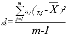
where xj is the mean of sample j, and x is the grand mean.
The numerator of the variance between is the sum of the squares of the distance between each x’s sample mean and the grand mean. It is simply a summing of one of those sources of variance across all of the observations.
The variance within is found by:
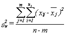
Double sums need to be handled with care. First (operating on the inside or second sum sign) find the mean of each sample and the sum of the squares of the distances of each x in the sample from its mean. Second (operating on the outside sum sign), add together the results from each of the samples.
The strategy for conducting a one-way analysis of variance is simple. Gather m samples. Compute the variance between the samples, the variance within the samples, and the ratio of between to within, yielding the F-score. If the F-score is less than one, or not much greater than one, the variance between the samples is no greater than the variance within the samples and the samples probably come from populations with the same mean. If the F-score is much greater than one, the variance between is probably the source of most of the variance in the total sample, and the samples probably come from populations with different means.
The details of conducting a one-way ANOVA fall into three categories: (1) writing hypotheses, (2) keeping the calculations organized, and (3) using the F-tables. The null hypothesis is that all of the population means are equal, and the alternative is that not all of the means are equal. Quite often, though two hypotheses are really needed for completeness, only Ho is written:
[latex]H_o: m_1=m_2=\ldots=m_m[/latex]
Keeping the calculations organized is important when you are finding the variance within. Remember that the variance within is found by squaring, and then summing, the distance between each observation and the mean of its sample. Though different people do the calculations differently, I find the best way to keep it all straight is to find the sample means, find the squared distances in each of the samples, and then add those together. It is also important to keep the calculations organized in the final computing of the F-score. If you remember that the goal is to see if the variance between is large, then its easy to remember to divide variance between by variance within.
Using the F-tables is the third detail. Remember that F-tables are one-tail tables and that ANOVA is a one-tail test. Though the null hypothesis is that all of the means are equal, you are testing that hypothesis by seeing if the variance between is less than or equal to the variance within. The number of degrees of freedom is m-1, n-m, where m is the number of samples and n is the total size of all the samples together.
Example #2
The young bank manager in Example 1 is still struggling with finding the best way to staff her branch. She knows that she needs to have more tellers on Fridays than on other days, but she is trying to find if the need for tellers is constant across the rest of the week. She collects data for the number of transactions each day for two months. Here are her data:
Mondays: 276, 323, 298, 256, 277, 309, 312, 265, 311
Tuesdays: 243, 279, 301, 285, 274, 243, 228, 298, 255
Wednesdays: 288, 292, 310, 267, 243, 293, 255, 273
Thursdays: 254, 279, 241, 227, 278, 276, 256, 262
She tests the null hypothesis:
[latex]H_o: m_m=m_{tu}=m_w=m_{th}[/latex]
and decides to use α - .05. She finds:
m = 291.8
tu = 267.3
w = 277.6
th = 259.1
and the grand mean = 274.3
She computes variance within:
[(276-291.8)2+(323-291.8)2+...+(243-267.6)2+...+(288-277.6)2+...+(254-259.1)2]/[34-4]=15887.6/30=529.6
Then she computes variance between:
[9(291.8-274.3)2+9(267.3-274.3)2+8(277.6-274.3)2+8(259.1-274.3)2]/[4-1]
= 5151.8/3 = 1717.3
She computes her F-score:
![]()
Figure 6.3 Interactive Excel Template for One-Way ANOVA - see Appendix 6.
You can enter the number of transactions each day in the yellow cells in Figure 6.3, and select the α. As you can then see in Figure 6.3, the calculated F-value is 3.24, while the F-table (F-Critical) for α - .05 and 3, 30 df, is 2.92. Because her F-score is larger than the critical F-value, or alternatively since the p-value (0.036) is less than α - .05, she concludes that the mean number of transactions is not equal on different days of the week, or at least there is one day that is different from others. She will want to adjust her staffing so that she has more tellers on some days than on others.
Summary
The F-distribution is the sampling distribution of the ratio of the variances of two samples drawn from a normal population. It is used directly to test to see if two samples come from populations with the same variance. Though you will occasionally see it used to test equality of variances, the more important use is in analysis of variance (ANOVA). ANOVA, at least in its simplest form as presented in this chapter, is used to test to see if three or more samples come from populations with the same mean. By testing to see if the variance of the observations comes more from the variation of each observation from the mean of its sample or from the variation of the means of the samples from the grand mean, ANOVA tests to see if the samples come from populations with equal means or not.
ANOVA has more elegant forms that appear in later chapters. It forms the basis for regression analysis, a statistical technique that has many business applications; it is covered in later chapters. The F-tables are also used in testing hypotheses about regression results.
This is also the beginning of multivariate statistics. Notice that in the one-way ANOVA, each observation is for two variables: the x variable and the group of which the observation is a part. In later chapters, observations will have two, three, or more variables.
The F-test for equality of variances is sometimes used before using the t-test for equality of means because the t-test, at least in the form presented in this text, requires that the samples come from populations with equal variances. You will see it used along with t-tests when the stakes are high or the researcher is a little compulsive.
