Chapter 3. Psychological Science
Interpreting Research
Amelia Liangzi Shi
Approximate reading time: 12 minutes
Learning Objectives
By the end of this section, you will be able to:
- Understand descriptive statistics and know how to produce them.
- Understand inferential statistics and why they are used.
Once data is collected from the research participants, a set of statistical analyses is conducted to interpret the results. Descriptive statistics organise and summarise some important properties of the data set. Researchers usually describe the central tendency and variability of a data set; this allows them to quickly make some basic interpretations about the results of a large sample of people. They may also use frequency distributions and histograms to visualize the data set. Inferential statistics provide researchers with the tools to make inferences about the meaning of the results, specifically about generalising from the sample they used in their research to the greater population that the sample represents. In experimental studies, researchers run inferential statistics to determine the likelihood that the effect of treatment is due to chance (and thus not meaningful). Generally, psychologists consider differences to be statistically significant if there is less than a five percent chance of observing them if the groups did not actually differ from one another. Stated another way, psychologists want to limit the chances of making false-positive claims to five percent or less.
Descriptive Statistics
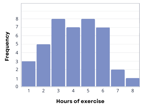
Let’s work through a hypothetical example to show how descriptive statistics help researchers to understand their data. Let’s assume that we have asked 40 people to report how many hours of moderate-to-intense physical activity they get each week. Let’s begin by constructing a frequency distribution of our hypothetical data that will show quickly and graphically what scores we have obtained.
| Hours of exercise | Number of participants |
|---|---|
| 1 | 3 |
| 2 | 5 |
| 3 | 8 |
| 4 | 7 |
| 5 | 8 |
| 6 | 7 |
| 7 | 2 |
| 8 | 1 |
We can now plot a histogram that will show the frequency (i.e., number of participants) as a function of exercise hours. Note how easy it is to see the shape of the frequency distribution of scores.
Many variables that interest psychologists have distributions where most of the scores are located near the centre of the distribution, the distribution is symmetrical, and it is bell-shaped. A data distribution that is shaped like a bell is known as a normal distribution. Normal distributions are common in human traits, such as intelligence, height, and shoe size. Relatively few people are either extremely high or low scorers, and most people fall somewhere near the middle.
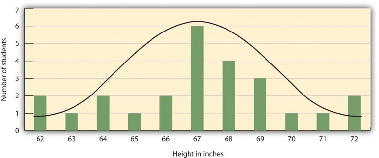
A distribution can be described in terms of its central tendency — that is, the point in the distribution around which the data are centred — and its variability or spread. The arithmetical average, or mean, denoted by the letter M, is the most commonly used measure of central tendency. It is computed by calculating the sum of all the scores of the variable and dividing this sum by the number of participants in the distribution, denoted by the letter N. In the data presented in Figure PS.14, the mean height of the students is 67.12 inches (170.48 cm).
In some cases, however, the data distribution is not symmetrical. This occurs when there are one or more extreme scores, known as outliers, at one end of the distribution. In Figure PS.15, you can see the variable of family income, which includes an outlier at a value of $3,800,000. In this case, the mean is not a good measure of central tendency. It appears from the histogram that the central tendency of the family income variable should be around $70,000. But again, because of the outlier, the mean family income is actually $223,960. The single very extreme income has a disproportionate impact on the mean, resulting in a value that does not well represent the central tendency.
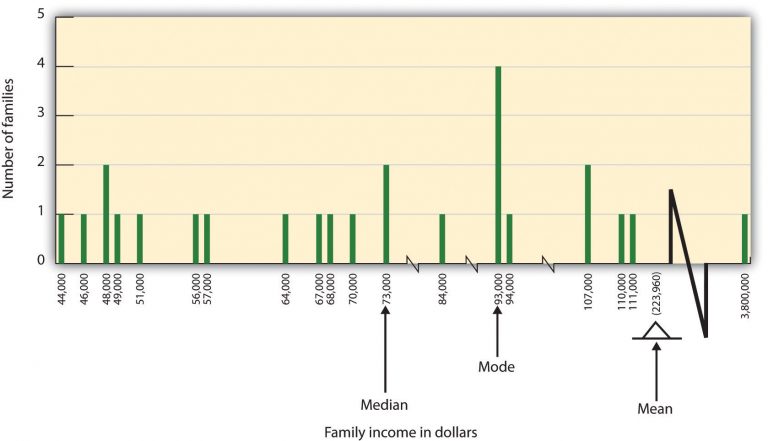
The median is used as an alternative measure of central tendency when distributions are not symmetrical. The median is the score in the centre of the distribution, meaning that 50% of the scores are greater than the median and 50% of the scores are less than the median. In our case, the median household income of $73,000 is a much better indication of central tendency than is the mean household income of $223,960.
A final measure of central tendency, known as the mode, represents the value that occurs most frequently in the distribution. You can see from the histogram that the mode for the family income variable is $93,000; it appears four times.
In addition to summarising the central tendency of a distribution, descriptive statistics convey information about how the scores of the variable are spread around the central tendency. Variability of a data set refers to the extent to which individual data points or values in the set differ from each other or from a central measure, such as the mean or median. In other words, it measures the spread or range of values within the data set. A data set with low variability has data points that are relatively close to each other, while a data set with high variability has data points that are more widely dispersed.
 This line graph forms a narrow bell shape around the central tendency. (b) This line graph forms a wide bell shape around the central tendency.")
One simple way to measure variability is to find the maximum score (i.e., the largest number in the data set) and the minimum score (i.e., the smallest number in the data set) and to compute the range of the variable as the maximum observed score minus the minimum observed score. In the previous example (Figure PS.14) , the range of height is 72 – 62 = 10.
The standard deviation, or SD, is the most commonly used measure of variability around the mean. Distributions with a larger standard deviation have more spread. Those with small deviations have scores that do not stray very far from the average score. Thus, standard deviation is a good measure of the average deviation from the mean in a set of scores. In the examples above, the SD of height is 2.74, and the SD of family income is 745,337. Standard deviation can be useful to compare the variability across samples. For example, a professor can keep track of student grades over many semesters. If the standard deviations are similar from semester to semester, this indicates that the amount of variability in student performance is fairly constant. A standard deviation that suddenly goes up indicates that there are more students with very low scores, very high scores, or both.
The standard deviation in the normal distribution has some interesting properties. Approximately 68% of the data fall within 1 standard deviation above or below the mean score: 34% fall above the mean, and 34% fall below. In other words, if a variable is normally distributed (e.g., height and IQ), approximately 2/3 of the population are within 1 standard deviation around the mean. Likewise, the 2 standard deviations account for 95% of the population, and the 3 standard deviations include almost everyone (99.73%).

Inferential Statistics
Descriptive statistics are useful in providing an initial way to describe and summarise a data set, but they are limited in informing us how meaningful the data are. The second step in analyzing data requires inferential statistics, such as t-tests. These tests are commonly used to assess the probability that observed results were due to chance. They allow researchers to generalise from the sample they used in their research to the greater population that the sample represents. Effect sizes are commonly used to estimate how large an effect has been obtained.
In the simplest, non-mathematical terms, the t-test is the researcher’s estimate of how likely it is that the observed group differences were statistically significant, as opposed to simply the result of chance. The t-test goes beyond just comparing means and can determine statistical significance even when the differences between experimental conditions are small; conversely, it might not find significance even when differences seem large. This shows the importance of considering inferential statistics like the t-test in evaluating the significance of experimental findings.
Typically, if a t-test shows that a result has a less than 5% probability of being due to chance alone, the result is considered to be real and to generalise to the population. If it shows that the probability of chance causing the outcome is greater than 5%, it is considered to be a non-significant result and, consequently, of little value; non-significant results are more likely to be chance findings and, therefore, should not be generalised to the population. Most researchers use p values to indicate the statistical significance: p < .05 means the probability of being caused by chance is less than 5% and therefore the result is “significant.” Although p values provide information about the presence of an effect, they are of little value for informing how large an effect is. For that, we need some measure of effect size. To learn more about why and how to report effect size, read this article: Using Effect Size—or Why the P Value Is Not Enough (Sullivan & Feinn, 2012).
In summary, statistics are an important tool in helping researchers understand the data that they have collected. Once the statistics have been calculated, the researchers interpret their results. Thus, while statistics are heavily used in the analysis of data, the interpretation of the results requires a researcher’s knowledge, analysis, and expertise.
Image Descriptions
Figure PS.14. Normal Distribution image description:
| Height in inches | Number of students |
|---|---|
| 62 | 2 |
| 63 | 1 |
| 64 | 2 |
| 65 | 1 |
| 66 | 2 |
| 67 | 6 |
| 68 | 4 |
| 69 | 3 |
| 70 | 1 |
| 71 | 1 |
| 72 | 2 |
Figure PS.15. Non-symmetrical Distribution image description:
| Family income in dollars | Number of families |
|---|---|
| $44000 | 1 |
| $46000 | 1 |
| $48000 | 2 |
| $49000 | 1 |
| $51000 | 1 |
| $56000 | 1 |
| $57000 | 1 |
| $64000 | 1 |
| $67000 | 1 |
| $68000 | 1 |
| $70000 | 1 |
| $73000 (Median) | 2 |
| $84000 | 1 |
| $93000 (Mode) | 4 |
| $94000 | 1 |
| $107000 | 2 |
| $110000 | 1 |
| $110000 | 1 |
| $3800000 | 1 |
Image Attributions
Figure PS.13. Original image created for this textbook and is under a CC BY-NC-SA license.
Figure PS.14. “Normal Distribution” is licensed under CC BY-NC-SA 3.0 license. The creator has asked that they not receive attribution.
Figure PS.15. “Non-Symmetrical Distribution” is licensed under CC BY-NC-SA 3.0 license. The creator has asked that they not receive attribution.
Figure PS.16. “Low Variability and High Variability” is licensed under CC BY-NC-SA 3.0 license. The creator has asked that they not receive attribution.
Figure PS.17. Empirical Rule by Dan Kernler is used under a CC BY-SA 4.0 license.
To calculate this time, we used a reading speed of 150 words per minute and then added extra time to account for images and videos. This is just to give you a rough idea of the length of the chapter section. How long it will take you to engage with this chapter will vary greatly depending on all sorts of things (the complexity of the content, your ability to focus, etc).
