20 Electrostatic Fields & Forces
Resources
- Video to Watch: Mechanical Universe - Episode 28 - Static Electricity
- Video to Watch: Mechanical Universe - Episode 29 - The Electric Field
- Extra Help: Charge Interactions Revisited
Equations Introduced and Used in this Topic:
- [latex]\vec{F}_{el}=\dfrac{kq_1{q}_2}{d^2}[/latex]
- [latex]\vec{F}_{el}=q\vec{E}[/latex]
- [latex]\vec{E}=\dfrac{kq}{d^2}[/latex]
- [latex]V=\dfrac{kq_1{q}_2}{d}[/latex]
[latex]q[/latex] = (± 1.602 × 10⁻¹⁹ C)(number of electrons/protons)
Bohr Radius [latex](a_0, r_{\text{Bohr}})=5.29177 × 10^{−11}\text{ m}[/latex]
Excited State Radius [latex]r =n^2 a_o[/latex]
[latex]\vec{F}=m\vec{a}[/latex]
Where…
- [latex]F[/latex] is generally the Net Force acting on the charged object
- [latex]F_{el}[/latex] is the Electrostatic Force, measured in newtons (N)
- [latex]E[/latex] is the Electric Field, measured in newtons per coulomb (N/C) or volts per metre (V/m)
- [latex]k[/latex] is the Coulomb's constant, measured in newton-metres squared per coulomb squared (N·m2/C2)
- [latex]q, q_1[/latex] & [latex]q_2[/latex] are the Charges you are studying, measured in coulombs (C)
- [latex]q[/latex] if negative indicates that it has an excess of electrons (or shortage of protons)
- [latex]q[/latex] if positive indicates that it has an excess of protons (or shortage of electrons)
- [latex]d[/latex] is the Distance away from the Charge Center, measured in metres (m)
- [latex]V[/latex] is the Potential Difference, measured in volts (V) or joules/coulombs (J/C)
- [latex]a[/latex] is the Acceleration of the object measured in metres per second squared (m/s2)
The static charge on an object can be calculated by the number of excess electrons or protons time ± 1.602 × 10⁻¹⁹ C
| Particle | Mass | Charge |
|---|---|---|
| Electron (e− or ß−) | 9.10938356(11) × 10−31 kg | −1.6021766208 × 10⁻¹⁹ C (−e) |
| Proton (p, p+ or N+) | 1.672621898(21) × 10−27 kg | +1.6021766208 × 10⁻¹⁹ C (+e) |
| Neutron (n, n0, N0) | 1.674927471(21) × 10−27 kg | 0 C |
| Alpha particle (α, α2+, He2+) | 6.644657230(82) × 10−27 kg | +3.2043532416 × 10⁻¹⁹ C (+2e) |
Important Constants (round to needed accuracy)
- Coulomb's constant: [latex]k[/latex] = 8.9875517873681764 × 10⁹ Nm2/C2
- Electron volt: 1 eV = 1.60217653(14) × 10−19 J
- Bohr Radius: (a0, rBohr) = 5.29177 × 10⁻¹¹ m
20.1 Electrostatic Forces
Equations Introduced or Used for this Section:
- [latex]\vec{F}_{el}=\dfrac{kq_1{q}_2}{d^2}[/latex]
- [latex]\vec{F}_{net}=m\vec{a}[/latex]
[latex]q[/latex] = (± 1.602 × 10⁻¹⁹ C)(number of electrons/protons)
Historical records indicate awareness of numerous electrical phenomenon for over 3000 years but the explanations of what it was quite different from how we understand it today. For instance, Thales of Miletus (624-546 BCE) thought that we were seeing the soul of a piece of amber that when rubbed on a fur it would attracted small objects. Likewise, lightning, St Elmo’s Fire and the electric ray all were well known electrical phenomena that had equally mystic nature.
Different from the study of mathematics and astronomy, the first recorded study of electrical phenomenon was published by William Gilbert (1544-1603) three years before his death from what is believed to have been the bubonic plague. The name for electricity came from Gilbert's use of the Latin word “electrica” (ἤλεκτρον) meaning “like amber”. While electrica had been used since the 13th century, Gilbert defined the name respecting its attractive or repulsive properties.
From Gilbert’s work, three rules of electrostatics were developed:
- There are only two kinds of electric charge
- Two objects charged alike (having the same kind of charge) repel each other
- Two objects charged oppositely attract each other.
Explaining the nature of charged objects was more challenging. Gilbert speculated that the “amber effect” was the result of the effluvium (small particles that flowed from one charged object to another that did not have any mass or volume). Over the next century, multiple small advances were made by numerous philosopher/scientists with one, Charles François de Cisternay du Fay (1698-1739), proposing that there were two types of electric charge: a positive charged fluid and a negative charged fluid. However, it was Benjamin Franklin (1706-1790) who formulated that electric charge was but a single fluid, not that an object having an excess of this fluid was positively charged and an object having a deficit of this fluid was negatively charged.
We now know that the Franklin one-fluid model is fundamentally correct in that it is the electron that can be understood as the source of electric charge. Because of this construct, everything in conventional electricity is defined in terms of the movement of this excess charge. However it was not until the late 1890’s that evidence accumulated to support what electric charge actually was. By this time, the battery, lightbulb, telephone and a host of other electrical inventions had been created, and all were understood using Franklin’s concept of the movement of excess fluid. The legacy of Franklin’s understanding can still be found in electrical terminology, including: positive and negative charge, charging and discharging, conductors and condensers, the lightning rod, and the flow of electric charge called electric current. Franklin[2] and William Watson (1715-1787) both proposed the conservation of electric charge. This concept was later interpreted as an isolated system wherein the net charge remains constant and, if matter is created or destroyed, charge is created and destroyed in equal amounts.
Quantifying the force that exists between similar or oppositely charged objects was proposed by Joseph Priestly (1733-1804) to follow an inverse square law as had been proposed by Isaac Newton for gravity. Priestly posited this relationship in his 700 page book The History and Present State of Electricity (1767). Priestly's inverse square law became formalized by Charles-Augustin de Coulomb (1736-1806), who demonstrated evidence of its authenticity using a device called the torsion balance. Coulomb later was able to demonstrate that an inverse square law relationship also existed between the poles of bar magnets.
In algebraic form, Coulomb’s Law is stated as:
[latex]\vec{F}_{el}=\dfrac{kq_1{q}_2}{{d}^2}[/latex]
Where…
- [latex]k[/latex] = 8.9875517873681764 × 10⁹ Nm2/C2 (Coulomb’s constant)
- [latex]q[/latex] = (± 1.602 × 10⁻¹⁹ C) (number of electrons/protons)
- [latex]d[/latex] = the distance between the charge centres (measured in metres)
Example 20.1.1
A small plastic sphere has a charge of −10−14 C.
- Does it have an excess or a deficit of electrons on it?
- How many electrons?
Solution
- Since the sphere has a negative charge, it has an excess of electrons.
- Data:
- [latex]q[/latex] = (± 1.602 × 10⁻¹⁹ C)
- [latex]n[/latex] = Find
Solution:
- [latex]q[/latex] = (± 1.602 × 10⁻¹⁹ C)(number of electrons/protons)
- −10−14 C = (+ 1.602 × 10⁻¹⁹ C)([latex]n[/latex])
- [latex]n[/latex] = −10−14 C ÷ (− 1.602) × 10−19 C
- [latex]n[/latex] = 62400 electrons (≈ 60000 e−)
Example 20.1.2
What is the magnitude and direction of the force acting on a charge of +4.2 µC, 5.0 mm away from a charge of +4.5 µC?
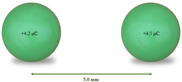
Solution
Data:
- [latex]F_{el}[/latex] = Find
- [latex]k[/latex] = 8.99 × 10⁹ Nm2/C2
- [latex]q_1[/latex] = 4.2 × 10⁻⁶ C
- [latex]q_2[/latex] = 4.5 × 10⁻⁶ C
- [latex]d[/latex] = 5.0 × 10⁻³ m
Solution:
- [latex]\vec{F}_{el}=\dfrac{kq_1{q}_2}{\text{d}^2}[/latex]
- [latex]\vec{F}_{el}=\dfrac{(8.99\times10^9 \text{ Nm}^2\text{/C}^2)(4.2\times10^{-6}\text{ C})(4.5\times10^{-6})}{(5.0\times10^{-3}\text{ m})^2}[/latex]
- [latex]\vec{F}_{el}[/latex] = 6800 N directed away from each other (both are positive charges)
Example 20.1.3
 The double-ionized lithium atom consists of one electron (e−) orbiting a core of three protons (p+) and three or four neutrons. If its average orbital radius is 0.0167 nm, what is the electrostatic force that exists between the electron and the core?
Solution
- [latex]\vec{F}_{el}=\dfrac{kq_1{q}_2}{d^2}[/latex]
- [latex]\vec{F}_{el}=\dfrac{(8.99\times10^9\text{ Nm}^2\text{/C}^2)(3)(4.5\times10^{-6})}{(0.0167\times10^{-9}\text{ m})^2}[/latex]
- [latex]\vec{F}_{el}[/latex] = 2.48 × 10⁻⁹ N (attractive)
Example 20.1.4
What is the acceleration of the single electron orbiting the three protons in the lithium atom described above? (Use the lowest energy level radius of 0.0167 nm.)
Solution
Data:
- [latex]a[/latex] = Find
- [latex]\vec{F}_{el}[/latex] = 2.48 × 10⁻⁶ N
- [latex]m[/latex] = 9.11 × 10⁻³¹ N
Solution:
- [latex]\vec{F}_{net}=\vec{F}_{el}[/latex]
- [latex]m\vec{\text{a}}[/latex] = 2.48 × 10⁻⁶ N
- (9.11 × 10−39 kg)([latex]\vec{a}[/latex]) = 2.48 × 10⁻⁶ N
- [latex]\vec{a}[/latex] = 2.7 × 10−39 m/s2... (towards the core)
Example 20.1.5
What is the distance that an electron would have to be away from the lithium core described above to experience an electrostatic force equal to its weight?
Solution
Data:
- [latex]m[/latex] = 9.11 × 10⁻³¹ kg
- [latex]q[/latex] = 1.602 × 10⁻¹⁹ C
- [latex]k[/latex] = 8.99 × 10⁹ Nm2/C2
- [latex]g[/latex] = 9.80 m/s2
- [latex]d[/latex] = Find
Solution:
- Use [latex]w=\vec{F}_{el}[/latex]
- [latex]mg=\dfrac{kq_1{q}_2}{d^2}[/latex]
- (9.11 1 × 10⁻³¹ kg)(9.80 m/s2) = [latex]\dfrac{(8.99\times10^9\text{ Nm}^2\text{/C}^2)(1.602\times10^{-19}\text{ C})^2}{d^2}[/latex]
- [latex]d^2[/latex] = 6.9 × 10⁻²⁸ N/m2 ÷ 8.9 × 10⁻³⁰ N
- [latex]d[/latex] = 8.8 m
Exercise 20.1
- A ping pong ball has a charge of −10−12 C.
- Does it have an excess or a deficit of electrons on it?
- How many electrons?
- What is the magnitude and direction of the electrostatic force acting on a charge of + 5.0 × 10⁻⁸ C that is 5.0 cm away from a charge of + 4.0 × 10⁻⁹ C?
- The hydrogen atom consists of an electron (e−) and a proton (p+). If their average separation is 5.29 × 10⁻¹¹ m what is the electrostatic force that exists between them?
- Two charged objects, one of +5.0 × 10⁻⁷ C and the other of −2.0 × 10⁻⁷ C, attract each other with an electrostatic force of 100 N. How far apart are they?
- The hydrogen atom has been extensively studied and has been responsible for scientists to be able to both create and understand the atomic structure of atoms. Given that the average radius for the first three excited states are:
- 1st excited state is 2.12 × 10⁻¹⁰ m
- 2nd excited state is 4.76 × 10⁻¹⁰ m
- 3rd excited state is 8.46 × 10⁻¹⁰
Find the different electrostatic forces experience by the electron in the first and third excited states.
- What is the acceleration of an electron orbiting the proton in the hydrogen atom? (Use the Bohr Radius... Ground State Radius.)
- Two small metal pellets (mass of 7.5 × 10⁻⁴ kg) each have the same negative charge and repel each other with an electrostatic force of 1.5 × 10⁻⁸ N when 5.0 mm apart.
- What would they accelerate with if they were free to move?
- How many electrons are on each of them?
- A singly ionized helium atom composed of a core that has 2 protons and 2 neutrons, has one electron orbiting. At what rate are the core and the electron accelerating towards each other if the electron maintains an average distance of 2.21 × 10⁻¹¹ m from the core?
- What is the distance an electron would have to be from a proton to have an acceleration of 10 g’s?
- What is the distance that an electron would have to be from a proton to experience an electrostatic force equal to its weight?
20.2 Electric Fields (Point Charges)
- Extra Help: Electric Field Intensity
- Extra Help: Electric Field Lines
Equations Introduced or Used for this Section:
- [latex]\vec{E}=\dfrac{kq}{d^2}[/latex]
- [latex]\vec{F}_{el}= q\vec{E}[/latex]
- [latex]\vec{F}= m\vec{a}[/latex]
- [latex]\vec{F}_{el}=\dfrac{kq_1{q}_2}{d^2}[/latex]
ike the concept of gravitational fields covered in Chapter 17.2, electrostatics share a similar concept of electric field (also magnetic fields). Historically, the first reference to such a concept was by Gilbert when he was describing the sphere of influence of a charged object. The equation quantifying the electric field can be derived in similar fashion to the derivation of the gravitational field. This can be shown as follows:
[latex]\vec{F}_{el}= q\vec{E}[/latex] is equated to [latex]\vec{F}_{el}=\dfrac{kq_1{q}_2}{d^2}[/latex]
This means that [latex]q\vec{E}=\dfrac{kq_1{q}_2}{d^2}[/latex]
cancelling out the common charge leaves us with... E = [latex]\dfrac{kq_1}{d^2}[/latex]
The direction of the electric field as defined by a negative or positive sign depends on the net charge of the object... Is the overall charge of the object negative or positive, and how it would react on a small positive test charge placed in the electric field . This means that the electric field can be written as either a positive or a negative quantity. In practice, many will ignore the positive and negative signs and just draw the field as attractive if the net charge is negative or repulsive if the net charge is positive.
[latex]\vec{E}=\pm\dfrac{kq_1}{d^2}[/latex]
The units of electrical field strength are N/C. This equation relates to the electric field at any distance away from a charged object and is a inverse square law relationship.
[latex]\vec{E}[/latex] ∝ [latex]\dfrac{1}{d^2}[/latex]
When we look at the electric field strength as we move inside the charged object’s surface, the electric field strength drops to zero. Anything inside the charged object is shielded from the electric field; this is why a radio signal on a vehicle fades out when driving through a tunnel or inside the metal frame of a bridge.
[latex]\vec{E}[/latex] = 0 N/C
Electric fields can have multiple variations of positive and negatively charged objects. Examples showing field lines of various combinations of positive and negative charges are shown below.
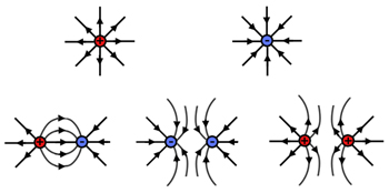
These field lines show the direction of the force that a small positive test charge would experience if placed near these charged objects. Also note that as the field lines get closer together, the field strength gets stronger and as the field lines move farther apart from each other, the field weakens. 
Example 20.2.1
What is the electric field at a distance of 15 cm above a small metal sphere that has a deficit of 420 million electrons?
Solution
Data:
- [latex]E[/latex] = Find
- [latex]k[/latex] = 8.99 × 10⁹ Nm2/C2
- [latex]q[/latex] = (420 × 106)(1.602 × 10⁻¹⁹ C)
- [latex]d[/latex] = 0.15 m
Solution:
- [latex]\vec{E}=\dfrac{kq_1}{d^2}[/latex]
- [latex]\vec{E}=\dfrac{(8.99\times10^9\text{ Nm}^2\text{/C}^2)(420\times10^6)(1.602\times10^{-19}\text{ C})}{(0.15\text{ m})^2}[/latex]
- [latex]\vec{E}[/latex] = 26.9 N/C (≈ 27 N/C)
Example 20.2.2
The electric field at a certain distance from a charged sphere is 200 000 N/C directed away from the sphere.
- What force would this exert on a singly ionized lithium atom ([latex]m[/latex] = 1.15 × 10⁻²⁶ kg and [latex]q[/latex] = −e)?
- What is the acceleration of this ion?
Solution
- [latex]\vec{F}_{el}=q\vec{E}[/latex]
[latex]\vec{F}_{el}[/latex] = (1.602 × 10⁻¹⁹ C)(200000 N/C)
[latex]\vec{F}_{el}[/latex] = 3.2 × 10⁻¹⁴ N - [latex]\vec{F}_{net}=\vec{F}_{el}[/latex]
[latex]m\vec{a}=q\vec{E}[/latex]
(1.15 × 10⁻²⁶ kg)[latex]\vec{a}[/latex] = (1.602 × 10⁻¹⁹ C)(200000 N/C)
[latex]\vec{a}[/latex] = 3.2 × 10⁻¹⁴ N ÷ 1.15 × 10⁻²⁶ kg
[latex]\vec{a}[/latex] = 2.8 × 10¹² m/s2 (away form the ion)
Example 20.2.3
An electron and a proton both experience an electric field strength of 50 N/C. What is the difference in accelerations that they experience? (Vector signs are included to identify the difference between Electric Field and Energy.)
Solution
The electron...
- [latex]\vec{F}_{net}=\vec{F}_{el}[/latex]
- [latex]m\vec{a}=q\vec{E}[/latex]
- (9.11 × 10⁻³¹ kg) [latex]\vec{a}[/latex] = (1.602 × 10⁻¹⁹ C)(50 N/C)
- [latex]\vec{a}[/latex] = 8.01 × 10⁻¹⁸ N ÷ 9.11 × 10⁻³¹ kg
- [latex]\vec{a}[/latex] = 8.79 × 10¹² m/s2
The proton...
- [latex]\vec{F}_{net}=\vec{F}_{el}[/latex]
- [latex]m\vec{a}=q\vec{E}[/latex]
- (1.67 × 10⁻²⁷ kg) [latex]\vec{a}[/latex] = (1.602 × 10⁻¹⁹ C)(50 N/C)
- [latex]\vec{a}[/latex] = 8.01 × 10⁻¹⁸ N ÷ 1.67 × 10⁻²⁷ kg
- [latex]\vec{a}[/latex] = 4.80 × 10⁹ m/s2
The difference...
- [latex]\Delta\vec{a}=\vec{a}_{e-}-\vec{a}_{p+}[/latex]
- [latex]\Delta\vec{a}[/latex]= 8.79 × 10¹² m/s2 − 4.80 × 10⁹ m/s2
- [latex]\Delta\vec{a}[/latex] = 8.78 × 10¹² m/s2
Exercise 20.2
- What is the strength and direction of the electric field at a distance of 5.29 × 10⁻¹¹ m away from a proton?
- What is the electric field at a distance of 20 cm above a small metal sphere that has a deficit of 100 million electrons?
- What strength of electric field is needed to exert a force on a proton equal to its weight?
- The electric field at a certain distance from a charged sphere is 500000 N/C from the sphere.
- What force would this exert on a neon ion ([latex]m[/latex] = 3.3 × 10⁻²⁶ kg and [latex]q[/latex] = −e)?
- What is the acceleration of this ion?
- An electron is present in an electric field of 104 N/C.
- Find the force acting on this electron.
- What is this electron’s acceleration?
- An electron is accelerated towards an alpha particle (charge is +2 e). How close does it get before it experiences an electric field of 1.0 N/C?
- What strength of electric field is needed to accelerate an electron at one million gravities?
- What is the change in the electric field strength as an object moves from 20 nm to 2.0 nm towards an alpha particle?
20.3 The Hydrogen Atom
| Particle | Mass | Charge |
|---|---|---|
| Electron (e− or ß−) | 9.10938356(11) × 10−31 kg | −1.6021766208 × 10⁻¹⁹ C (−e) |
| Proton (p, p+ or N+) | 1.672621898(21) × 10−27 kg | +1.6021766208 × 10⁻¹⁹ C (+e) |
Equations Introduced or Used for this Section:
Bohr Radius [latex](a_0, r_{\text{Bohr}})=5.29177 × 10^{−11}\text{ m}[/latex]
Excited State Radius [latex]r =n^2 a_o[/latex]
- [latex]F_{el}=\dfrac{kq_1{q}_2}{d^2}[/latex]
- [latex]F_{c}=\dfrac{mv^2}{r}[/latex]
- [latex]E_k=\dfrac{1}{3}mv^2[/latex]
- [latex]p=mv[/latex]
The hydrogen atom is important to an understanding of both the structure of atoms and the quantum nature of matter. One of the first clues to the nature of the hydrogen atom came from the emission spectrum (the specific colors) that hydrogen gas emits when heated. In 1885 Jacob Balmer (1825-1898) discovered that the visible wavelengths associated with the specific emitted colors fit a simple formula. By manipulating the formula, Balmer found other series of wavelengths, both visible and invisible.
Ernest Rutherford (1871-1937) solved the remaining part of the mystery of the nature of atomic structure. Rutherford worked at three universities (including McGill in Montreal) and later at the Cavendish Laboratory. He discovered that atoms were mostly space, with an inner hard core surrounded by orbiting electrons, much like planets orbiting a sun at the centre. This concept, the Rutherford Planetary Model of the Atom, can be added to his concepts of alpha, beta and gamma rays, protons and half-life radioactivity.
Combining the results of Balmer and Rutherford, Niels Bohr (1885-1962) used the energy of the emitted light spectra to come up with a model of the atom that certain average orbitals around the nucleus or core were allowed. Bohr’s work predicted the size of the hydrogen atom and initiated an understanding of the nature of the movement of the electron around the atom. Rutherford’s Planetary Model and Balmer’s emission spectra were now grounded in a common conceptual understanding.
In less than two decades, Werner Heisenberg (1901-1976), Paul Dirac (1902-1984) and Wolfgang Pauli (1900-1958) together laid out the foundations of quantum mechanics by focusing on the frequencies and intensities of the hydrogen spectra transitions, and the elliptical effect of the electron orbits on the hydrogen spectra, with the mathematical genius to put it all together.
The following questions relate to the Hydrogen Atom.
Example 20.3.1
- What is the strength of the electrostatic force between an electron and a proton separated by a distance of 2.12 × 10⁻¹⁰ m (1st excited state)?
- [latex]F_{el}=\dfrac{kq_1{q}_2}{d^2}[/latex]
- [latex]\vec{E}=\dfrac{(8.99\times10^9\text{ Nm}^2\text{/C}^2)(1.602\times10^{-19}\text{ C})(1.602\times10^{-19}\text{ C})}{(2.12\times10^{-10}\text{ m})^2}[/latex]
- [latex]\vec{E}[/latex] = 5.13 × 10⁻⁹ N
- Balancing the centripetal force to the electrostatic force for the hydrogen atom, calculate the speed of an electron that would be orbiting the proton (1st excited state).
- [latex]F_{c}=\dfrac{mv^2}{r}\qquad\qquad F_{el}=\dfrac{kq_1{q}_2}{d^2}[/latex]
- Therefore... [latex]\dfrac{mv^2}{r}=\dfrac{kq_1{q}_2}{d^2}[/latex] Cancel out the common distance & isolate v2
- Yields... [latex]v^2=\dfrac{kq_1{q}_2}{dm}[/latex]
- [latex]{v}^2=\dfrac{(8.99\times10^9\text{ Nm}^2\text{/C}^2)(1.602\times10^{-19}\text{ C})(1.602\times10^{-19}\text{ C})}{(2.12\times10^{-10}\text{ m})(9.11\times10^{-31}\text{ kg}}[/latex]
- [latex]v^2[/latex] = 1.19 × 10¹² m2/s2
- [latex]v[/latex] = 1.09 × 10⁶ m/s
- Calculate the kinetic energy and the momentum of this orbiting electron (1st excited state).
- [latex]E_k[/latex] = ½mv²
- [latex]E_k[/latex] = ½(9.11 × 10⁻³¹ kg)(1.09 × 10⁶ m/s)2
- [latex]E_k[/latex] = 5.41 × 10⁻¹⁹ J or 3.4 eV
- [latex]p = mv[/latex]
- [latex]p[/latex] = (9.11 × 10⁻³¹ kg)(1.09 × 10⁶ m/s)
- [latex]p[/latex] = 9.9 × 10⁻²⁵ Ns
Exercise 20.3
-
- What is the electrostatic force strength between an electron and a proton separated by 4.76 × 10⁻¹⁰ m (2nd excited state)?
- Balancing the centripetal force to the electrostatic force for the hydrogen atom calculate the speed of an electron that would be orbiting the proton (the hydrogen atom).
- Calculate the kinetic energy and the momentum of this orbiting electron.
- If an electron that is orbiting an alpha particle has a kinetic energy of 54.42 eV 114 what distance is this electron from the core? What is the centripetal force and the electrostatic force that is acting on this electron?
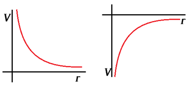
20.4 Electric Potential of Point Charges
The images below show the magnitude of the Electrical Potential of both a positive and negative charge as one moves away from the charge.
Equations Introduced or Used for this Section:
[latex]\Delta V[/latex] = ±[latex]\dfrac{kq}{d}[/latex] [latex]\Delta E[/latex] = ± [latex]q V[/latex]
Electric potential for charged objects is similar to the gravitational potential, in that instead of moving without friction through some displacement in a gravitational field, an object instead moves through a displacement inside an electrical field. There are two possibilities for this electric field: either the field is constant like the gravity one finds when moving through small changes in height on Earth, or the field varies similarly to the movement of a spaceship either towards or away from the Earth.
This results in two different equations for electric potential: the electric potential moving away from a charged object, or the electric potential in a constant electric field. This section looks at only the electric potential moving away from a charged object, that as such experiences a variable electric field.
Electric potential for a charged object can be used to find the energy change if the amount of charge moving through the potential difference is known. It is important to remember the distinction between electric potential and electric potential energy... They are different.
The equation for electric potential is one that is most useful in a number of physics situations that look at the energy required to remove an electron from an atom, or to move from one allowed orbital to another for an electron in orbit around an atom.
While the following examples relate to the hydrogen atom, applications of this equation extend far beyond this.
Example 20.4.1
What is the electric potential of an electron in its second excited state surrounding a hydrogen atom?
Solution
- [latex]V[/latex] = [latex]-\dfrac{kq}{d}[/latex]
- [latex]V[/latex] = [latex]-\dfrac{(8.99\times10^9\text{ Nm}^2\text{/C}^2)(1.602\times10^{-19}\text{ C})}{(2.12\times10^{-10}\text{ m})}[/latex]
- [latex]V[/latex] = − 6.79 N/m
Example 20.4.2
What is the electrical potential for a hydrogen atom between the average ground state radius (n = 1) 5.29 × 10⁻¹¹ m and (n = 4) average radius of 8.46 × 10⁻¹⁰ m.
Solution
This requires finding the change in electric potential between these two states...
- [latex]V_{n = 1}[/latex] = [latex]-\dfrac{kq}{d}[/latex]
- [latex]V[/latex] = [latex]-\dfrac{(8.99\times10^9\text{ Nm}^2\text{/C}^2)(1.602\times10^{-19}\text{ C})}{(5.29\times10^{-11}\text{ m})}[/latex]
- [latex]V[/latex] = − 27.2 N/m
- [latex]V_{n = 4}[/latex] = [latex]-\dfrac{kq}{d}[/latex]
- [latex]V[/latex] = [latex]-\dfrac{(8.99\times10^9\text{ Nm}^2\text{/C}^2)(1.602\times10^{-19}\text{ C})}{(8.46\times10^{-10}\text{ m})}[/latex]
- [latex]V[/latex] = − 1.70 N/m
- [latex]\Delta V = V_{n = 4} − V_{n = 1}[/latex]
- [latex]\Delta V[/latex] = − 1.70 N/m − (− 27.2 N/m) or 25.5 N/m
[latex]\Delta V[/latex] depends on the direction travelled (away or towards) and as such [latex]\Delta V[/latex] = ± 25.5 N/m
Exercise 20.4
- What is the electric potential of an electron in its ground state radius surrounding a hydrogen atom?
- What is the difference in electric potential to remove a proton at a distance of 25 µm from a charged sphere having a charge of 106 excess electrons?
- What is the difference in electrical potential for a hydrogen atom between the average ground state radius (n = 1) 5.29 × 10⁻¹¹ m and (n = 3) average radius of 4.76 × 10⁻¹⁰ m.
Exercise 20.5.1: Deep space research on hydrogen atoms
Deep space research on hydrogen atoms, suggest that electrons can orbit protons at distances as far as one metre apart (d = 1.0 m).
- What would be the orbital speed of this electron?
- What would be the kinetic energy of this electron?
Exercise Answers
20.1 Electrostatic Forces
-
- has extra electrons
- 6.25 × 10⁶ e−
- Repulsive force of 7.2 × 10⁻⁴ N
- Attractive force of 8.24 × 10⁻⁸ N
- 3.0 × 10⁻³ m
- 1st excited 5.12 × 10⁻⁹ N 3rd excited 3.2 × 10⁻¹⁰ N
- 9.03 × 10²² m/s2
- 2.0 × 10⁻⁵ m/s2
- 4.03 × 10⁷ e−
- 1.04 × 1024 m/s2 (electron) ac = 1.41 × 10²⁰ m/s2 (core)
- d = 1.61 m
- d = 5.1 m
20.2 Electric Fields (Point Charges)
- 5.15 × 10¹¹ N/C (away)
- 3.6 N/C away from Sphere
- 1.02 × 10⁻⁷ N/C upwards
-
- 8.0 × 10⁻¹⁴ N
- 2.4 × 10¹² m/s2
-
- 1.7 × 10⁻¹⁷ N
- 1.8 × 10¹³ m/s2
- 5.4 × 10⁻⁵ m
- 5.6 × 10⁻⁵ N/C
- 7.1 × 10⁸ N/C away
20.3 Hydrogen Atom
-
- 1.02 × 10⁻⁹ N
- 2.18 × 10⁶ m/s
- 1.99 × 10⁻²⁴ N/C
- [latex]F_{el}[/latex] = [latex]F_c[/latex] = 0.657 µN
20.4 Electric Potential
- [latex]V[/latex] = − 27.2 J/C
- [latex]V[/latex] = 57.5 J/C
- [latex]\Delta V[/latex] = 24.2 J/C
20.5.1 Deep space research on hydrogen atoms
- [latex]v[/latex] = 15.9 m/s
- 1.15 × 10⁻²⁸ J
Media Attributions
- "Point charge electric field patterns" by A-Level Physics Tutor is licensed under a CC BY-NC-ND licence.
- "Blausen 0615 Lithium Atom" by BruceBlaus is licensed under a CC BY-SA 4.0 licence.
- Example 20.2.1 image from College Physics by Paul Peter Urone, Roger Hinrichs, Kim Dirks and Manjula Sharma is licensed under a CC BY 4.0 licence.
- "Graph of electric potential" by user45220 of Stack Exchange is licensed under a CC BY-SA 3.0 licence.
- A-Level Physics Tutor - Electricity ↵
- Benjamin Franklin actually did his famous kite experiment in a thunderstorm in 1752, collecting electric charge in a capacitor which was known at that time as a Leyden Jar. Greater detail of this experiment can be found at: Kite experiment & Leyden jar ↵
