Lab 22: Alpine Glacial Processes
Crystal Huscroft and Katie Burles
In this lab you will be using your understanding of glacial processes to make observations and measurements documenting and predicting the consequences of climate change for a Canadian alpine glacier. You will learn how to analyze the characteristics of glaciers and glacial landforms from a variety of types and sources of satellite imagery.
Learning Objectives
After completion of this lab, you will be able to
- Make observations, identify, and appreciate the consequences of global warming for alpine glaciers.
- Analyze the characteristics of alpine glaciers in order to make predictions regarding the future survival of a glacier.
- Summarize and collate Geographic Information System (GIS) point, line, and area information from different platforms into a single GIS project.
- Acquire and interpret remotely sensed imagery.
- Communicate effectively regarding the impacts of global warming for British Columbian glaciers.
Pre-Readings
Introduction to Glacial Processes and Landforms
Understanding of the following key terms is required for this laboratory activity:
- Ablation zone
- Accumulation zone
- Annual ice horizon
- Cirque glacier
- Crevasses
- Equilibrium line
- Firn
- Glacial ice
- Glacier toe
- Moraine
- Snowline
- Trimline
- Valley glacier
If you are unfamiliar with any of these terms, look them up before continuing.
How to Determine Whether a Glacier Will Survive Current Climate
You will be asked to predict whether or not the glacier that you choose to study will survive within the current climate. Glaciers form and persist in areas where snow accumulation is consistently equal to or greater than snow and ice melt or sublimation (ablation). Glaciers that are in danger of disappearing will show evidence of insufficient snow accumulation to persist through the melt season. As described by Dr. Mauri Pelto on Glacier Survival website (please read) and Forecasting temperate alpine glacier survival from accumulation zone observations [PDF] (Pelto, 2010), the likelihood of a glacier’s survival can be assessed using the following visual clues in satellite imagery:
- Newly exposed rock outcrops in the accumulation zone. These rock outcrops may appear lighter than surrounding rock due to a lack of lichen growth on their surface.
- Lowering of the surface and a reduction in size of the upper margins of the glacier. This might also be indicated by light coloured rock margins around the edges of the glacier due to exposure of unvegetated (mostly lichen) rock and debris.
- Discontinuous snow cover in the accumulation zone. This may appear as patches of bare ice surrounded by snow.
- Less than a third snow cover over the glacier late in the melt season.
Video 22.1 captures a glaciologist, Dr. Mauri Pelto, applying the concepts above and performing the same type of analysis that you are asked to perform in this lab.
Video 22.1. Analyzing Sacagawea Glacier, Wind River Range Wyoming Survival.
Introduction to Sentinel 2 Imagery
In this lab, you will be analyzing false colour images captured by the Sentinel 2 satellite program. The Sentinel 2 program consists of twin satellites launched by the European Space Agency that are able to capture imagery of Earth at a resolution of 10-60 m. It consistently captures images between 56° S to 84° N every 5 days. Unlike our eyes, the satellite system can detect energy in the visible, near-infrared and shortwave infrared portions of the electromagnetic spectrum.
Although the satellites measure 13 spectral bands of reflected and emitted energy, false colour images using three specific bands of energy are excellent for studying glaciers because they are able to detect and differentiate ice and snow (Bands 11, 8A, 4). In these false colour images, snow appears light teal blue, ice appears dark teal blue, and water appears a very dark shade of blue.
Calculating Rates of Glacier Advance or Retreat
A rate is the amount of change in some quantity over a given period of time. In this lab we are interested in rates of advance or retreat of glaciers. This rate of movement is the rate of change (Δ) in distance per change in time. Glaciers move slowly, and so in this context the rate is commonly expressed in metres per year (m/y). The rate may be expressed as (Equation 22.1):
[latex]\text{Rate} = \dfrac{\Delta\text{ Distance}}{\Delta\text{ Time}}[/latex]
Glaciers generally advance each winter and retreat each summer. However, these annual advances and retreats may not be equal and so, over time, the glacier toe may, on average, advance or retreat. The average rate of advance or retreat is calculated by taking the total distance that the glacier toe has moved from the defined starting point/time and dividing it by the number of years that have elapsed.
For example, if the glacier has retreated 70 m in 35 years, using Equation 22.1,
[latex]\text{Rate} = \dfrac{\Delta\text{ Distance}}{\Delta\text{ Time}}[/latex]
[latex]\text{Rate} = \dfrac{70\text{ m}}{35\text{ y}} = 2\text{ m/y}.[/latex]
For a more detailed explanation of calculating rates, please refer to SERC Carleton's How do I calculate rates? Calculating changes through time in the geosciences.
Lab Exercises
In the exercises in this lab, you will choose a Canadian glacier and create a report consisting of satellite imagery and commentary regarding the likelihood of your glacier’s survival in the current climate. You will be accessing topographic and satellite information regarding your glacier from the following platforms so that you can discuss factors that have affected your glacier’s behaviour in terms of retreat and the likelihood that the glacier will survive current and future warming:
You will be guided to complete a lab report, which you will save as a PDF.
EX1: Describing a Canadian Alpine Glacier
Step 1: Choose a glacier.
- Open The Atlas of Canada - Toporama. Warning: this site loads slowly. If all you see is a link to GeoGratis, give it a few more moments to load a map. Explore the mountainous regions within Canada and choose an alpine glacier somewhere in Canada that you would like to study. In Toporama, you will see white areas denoting alpine areas, and then blue areas within the alpine areas denoting glacial ice. Glaciers are labelled in pink. Many Canadian glaciers are not named, however you may want to choose one that is for ease of reference.
- Determine the geographic grid coordinates (latitude and longitude) of your glacier in decimal degrees. In Toporama, this is done by clicking on the Menu drop-down in your Toporama viewer and the Get coordinates from the map tool. Click on your glacier and record the decimal degrees of your location.
- Ensure that there is good satellite imagery for your chosen glacier in Google Earth (Web). Open Google Earth (Web) and familiarize yourself with the navigation controls. In the search pane, type in your location in decimal degrees. Examine your glacier. It is best to choose an alpine glacier that is not too snow-covered in the Google Earth (Web) imagery so that the margins of the glacier are clearly visible. Also, cirque glaciers with a single outlet will be simpler to map than icefields with multiple outlets.
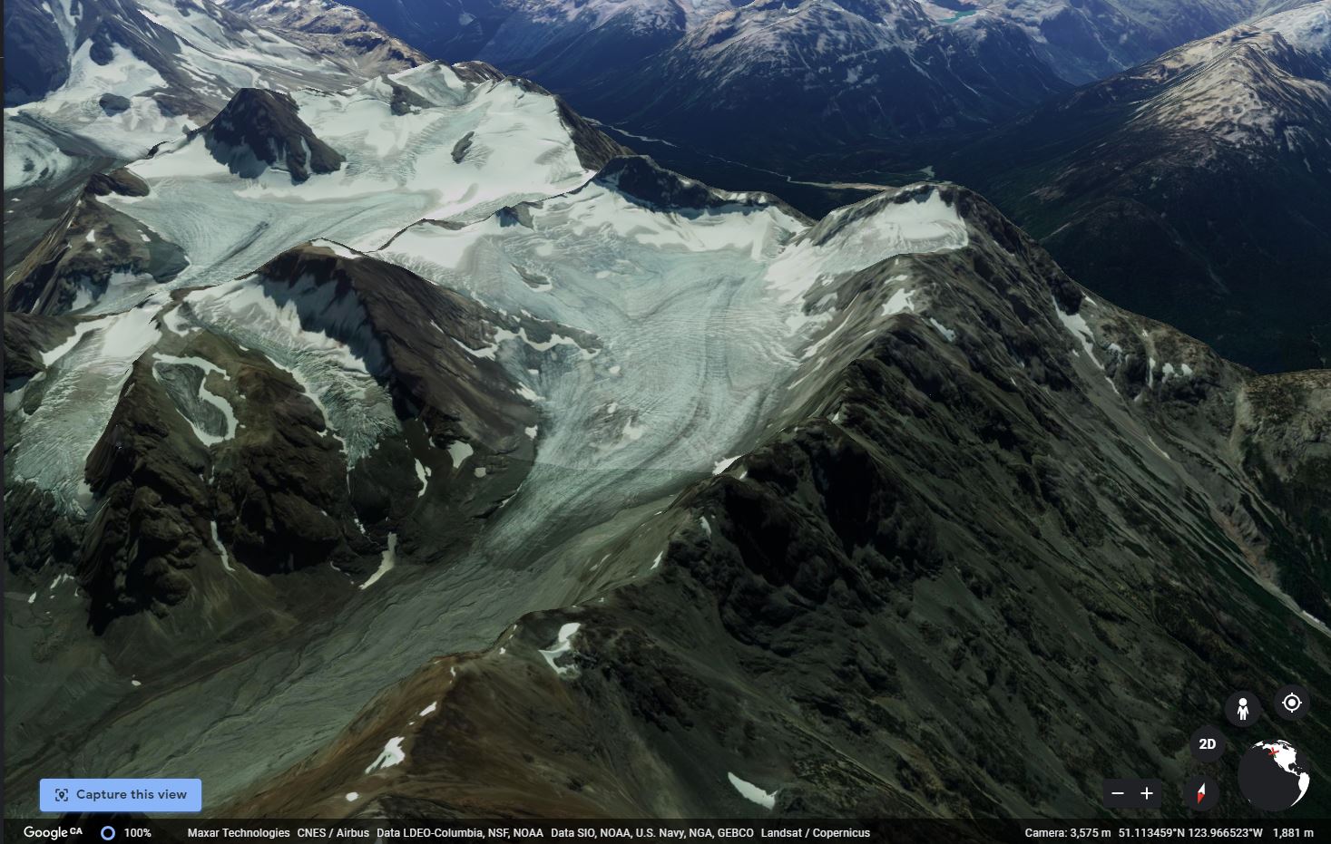
Step 2: Create an oblique 3D view of the glacier.
- Within Google Earth (Web), view your glacier in 3D. Tilt your view and navigate to a view of the glacier that gives a good perspective of the shape and steepness of your glacier, and enough of the adjacent topography to give the viewer an idea of the character of adjacent mountains.
- Create a screen capture of this view and save it as a JPEG file with a file name in the format <1_lastname_firstname_3D_image>. Your glacier should take up the majority of the center of the photo, so that it is obvious as to which glacier you are studying. This image will be Figure EX1.1 of your final lab report.
Step 3: Create a title page, slide and introduction (Figure EX1.1).
- The image in Step 2 will be the image for the title slide in your lab report and Google Earth (Web) presentation. Paste your image into a document that can later be saved as a PDF. Be sure to set up your document to landscape orientation. A sample student assignment can be found in Worksheets.
- Resize the image so that the image and caption for Figure EX1.1 can fit on one page in landscape orientation. Figure 22.1 provides an example.
- Write a figure caption in paragraph form that includes the following information:
- The glacier’s geographic grid coordinates in decimal degrees (latitude and longitude).
- The direction of view of the image. What direction (north, east, south, west) is the camera looking in the image you attached?
- The glacier’s name (if applicable). Many Canadian glaciers are not named. If you haven't already, you can check if your glacier has a name on The Atlas of Canada – Toporama website.
- A description of the glacier’s location relative to major landmarks like towns, lakes, highways. For example, 30 km northeast of Pemberton.
- The physiographic region the glacier is located within. Depending on the province or territory where you chose your glacier, you will need to refer to the following reports:
- British Columbia [PDF] (see Figure EX2.1 in this document)
- Alberta [PDF]
- Yukon [PDF]
- Nunavut and North West Territories (click to download the zip file of the Physiographic Regions of Canada GSCmap-a_1254A_e_1970_mn01 and open gscmap-as_1254A_e_1970.pdf from the doc folder).
- A description of the main bodies of water that the glacier meltwater feeds. At a minimum, you should indicate the name of the major streams that drain the glacier's meltwater and the receiving ocean. You can see this by tracing the flow of water from the glacier to an ocean using The Atlas of Canada – Toporama website.
- A description of why you chose the glacier. This is a short description and there is no wrong answer. Just be honest. Maybe you have seen this glacier, maybe you would like to travel there, or maybe your choice was completely random. If you have your own personal picture of the glacier that you would like to share, please include it as Figure EX1.1b. Your lab instructor would love to see it. You can choose to copyright it or release as Creative Commons by using this copyright builder.
- A description of the image source. The source of all images used in any report should be described.
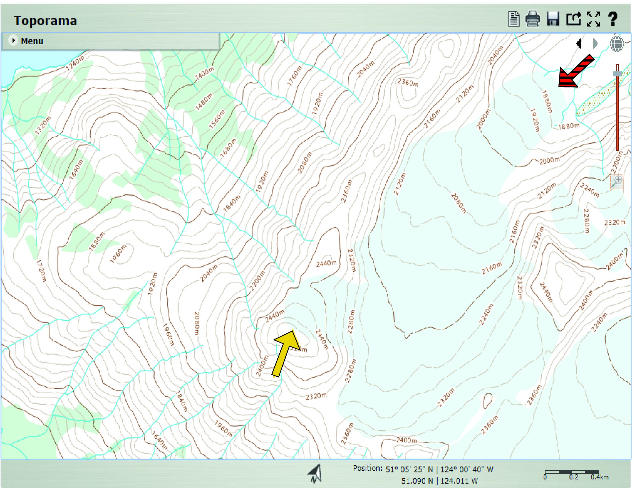
Step 4: Create and analyze a topographic map (Figure EX1.2).
- Figure EX1.2 of your report will be a topographic map with a north arrow and a scale bar of your glacier. Refer to the example Figure 22.2. In order to create the image, within The Atlas of Canada - Toporama, navigate back to a view of your glacier that captures the entire glacier from its source area.
- Using the Measuring and Drawing Tools menu on the left of your window, select a yellow pencil tool and draw a yellow arrow indicating the top elevation of your glacier's source area as well as a red arrow indicating the bottom elevation.
- Take a screen capture of your image that clearly shows the scale bar, the north arrow, the contours above and below your glacier, your yellow arrow, your red arrow and the north arrow.
- Save this image with a memorable file name. Paste this image onto the next page of your lab report in landscape view so that the image takes up most of the page, but still leaves room for the caption.
- Write a caption for your figure that includes the following:
- The aspect of the glacier. The aspect of the glacier indicates the direction that the glacier is facing or sloping down towards (north, east, west, or south-facing).
- The maximum and minimum elevation of the glacier based on interpolating between the contour lines.
- Whether or not the glacier originates from a cirque or valley glacier.
- The image source and the date accessed.
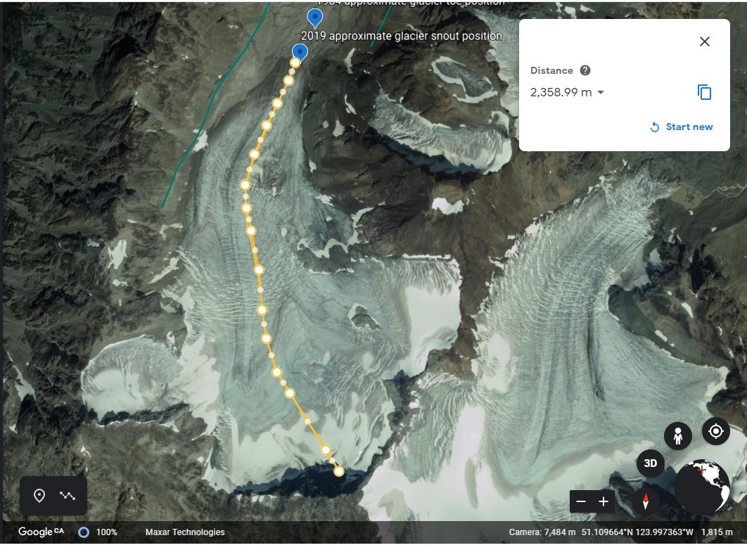
Step 5: Describe the length of the glacier (Figure EX1.3).
- In Google Earth (Web) start a new project and name it <Lastname Firstname Glacier Survival Lab>.
- Create a new line feature by digitizing a centerline for the glacier that extends from the approximate center of the upper extremity of the glacier to the lower extremity. Your line should follow the topography downwards. Your line should parallel the glacier flow direction and any downhill sloping debris bands. Name this feature Glacier length.
- Next, measure the length of this line with the Measure tool (ruler icon on the left side of your screen). While the value of the length is still displayed in a white box, take a screen capture of this measurement including the Google icon, and use the image as Figure EX1.3. Figure 22.3 provides an example.
- Write a caption that describes the length of the glacier to the nearest 10 m, the image source and the date accessed.
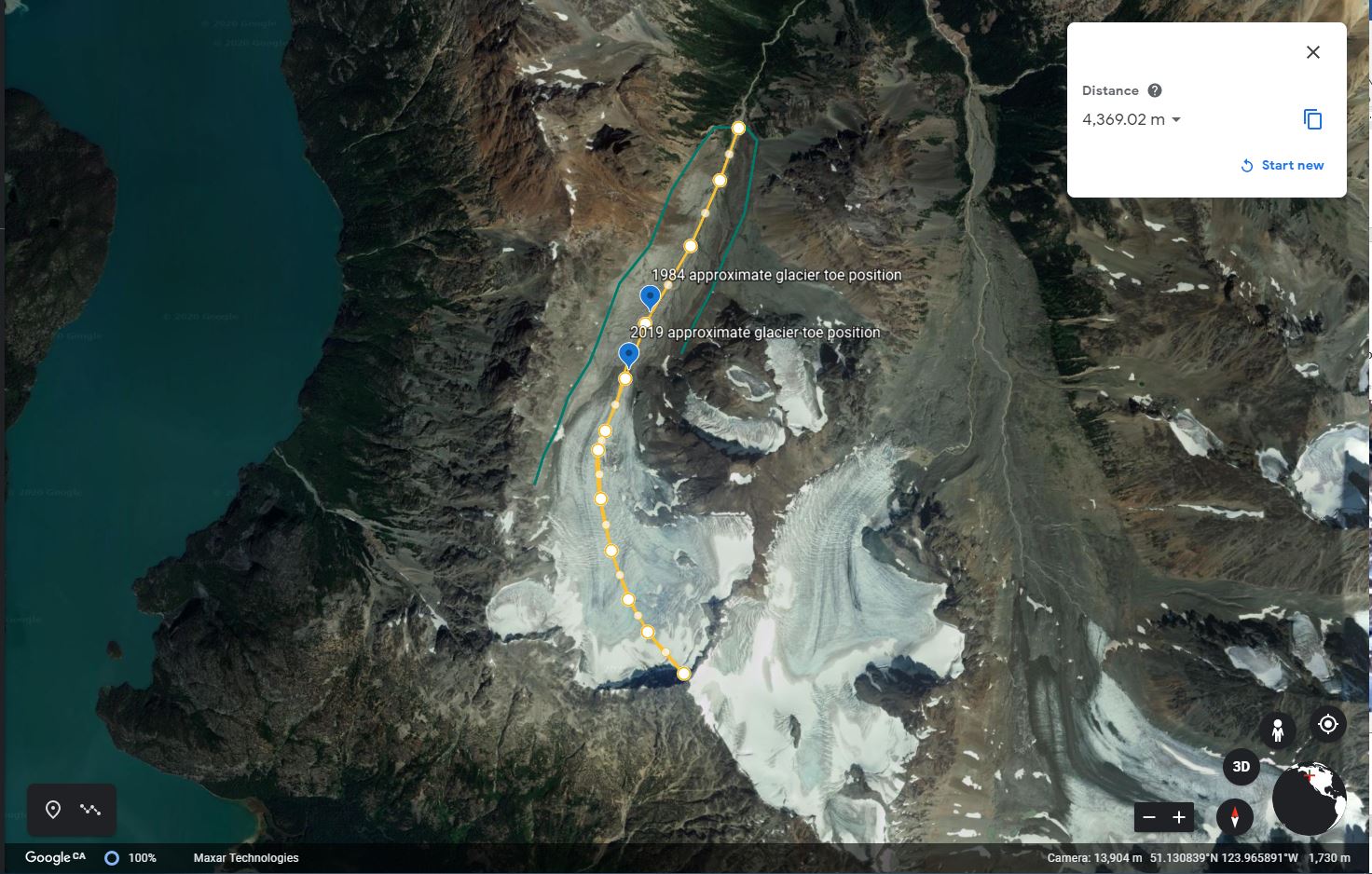
Step 6: Identify evidence of Little Ice Age Glacier extent (Figure EX1.4).
In this figure, you will try to depict any evidence of the past maximum extent of your glacier during the Little Ice Age. The Little Ice Age was a period of cool climate when glaciers in Europe and North America advanced from their current positions. The period spanning from 1100 Common Era (CE) to 1850 CE includes several series of advances. The evidence left on the landscape from these advances includes trimlines and moraines that wrapped around the edges and toe of the glacier.
- Zoom out from the view of your glacier to include the area down slope of the toe of your glacier. Using a green line, trace any features you see that could indicate how far your glacier once extended. If you do not see any indicators of past glacier extents (they may be obscured), you do not need to add any features.
- If you found clues as to prior glacier extents, measure how long the glacier once was. While the value of the measurement is still visible in a white box, create a screen capture and save the file as <4_Lastname_Little Ice Age>. If you did not see any evidence, create a screen capture of a view that supports your assertion that no features are evident and also save this file as <4_Lastname_Little Ice Age>. This will be Figure EX1.4 in your lab report. Figure 22.4 provides an example.
- Write a caption for Figure EX1.4 that indicates the types of clues you used and a measurement of how long the glacier may have extended during the Little Ice Age. If you did not find any clues, write a caption saying so and indicate the types of features that were absent.
EX2: Analyzing Glacier Change and Processes With Satellite Imagery
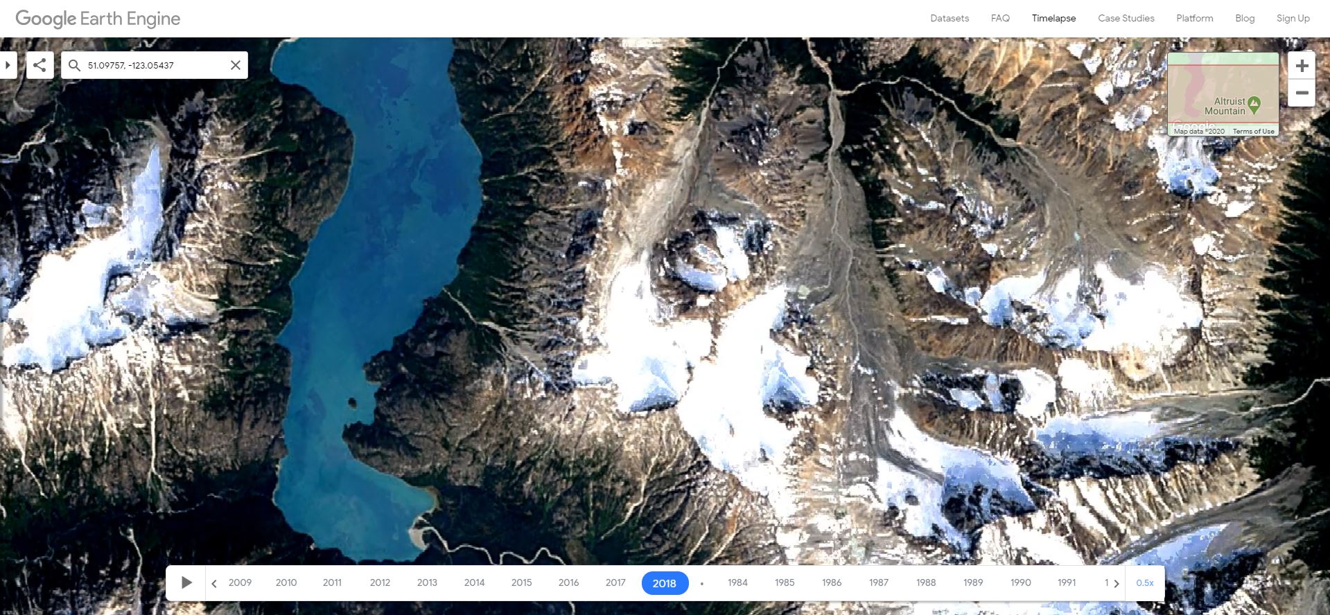
Step 1: Capture Google Earth Engine Timelapse imagery (Figures EX2.1 & EX2.2).
- Visit Google Earth Engine Timelapse and navigate to a large scale view of your glacier. It may load slowly, so give it a few moments. Zoom in as far as possible with your glacier in the centre of the view. Press the pause button on the lower left of the screen, then choose the earliest view (e.g., 1984) where the position of the toe of your glacier is visible. The earliest view should be before 1990.
- Create a screen capture of this view and save it with the file name <5_Lastname 1984 imagery>. Add the image to your document as Figure EX2.1.
- Write a caption for Figure EX2.1 indicating what the image is of, the date of the imagery and include a link to this view by using the Share Current View button and pasting it as the image source.
- Keeping the exact same view, repeat the previous three steps to produce Figure EX2.2 using the most recent imagery and save the screen capture with the file name <6_year_Lastname_Glacier_extent>. Figure 22.5 provides an example. Write a caption for Figure EX2.2 describing any changes you observe.
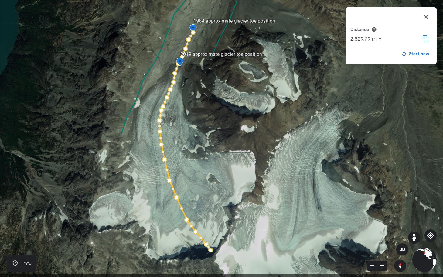
Step 2: Estimate the approximate location of the glacier toe in 1984 (creating a point feature and Figure EX2.3).
- Using landmarks visible in the earliest good imagery from Google Earth Engine Timelapse (this will most likely be 1984), add a point feature to your Google Earth project and move it to your best estimate of the location of the toe of the glacier in 1984. Use as many landmarks as possible to situate your point. Make sure your view is in 2D and it helps if you view both images at the same scale.
- For comparison, measure the length of the glacier you estimate in 1984 and create a screen capture of your measurement while the value of the measurement is still visible. Save this screen capture of Google Earth (Web) as <7_Lastname_1984_approximate_glacier_toe> (example provided as Figure 22.6).
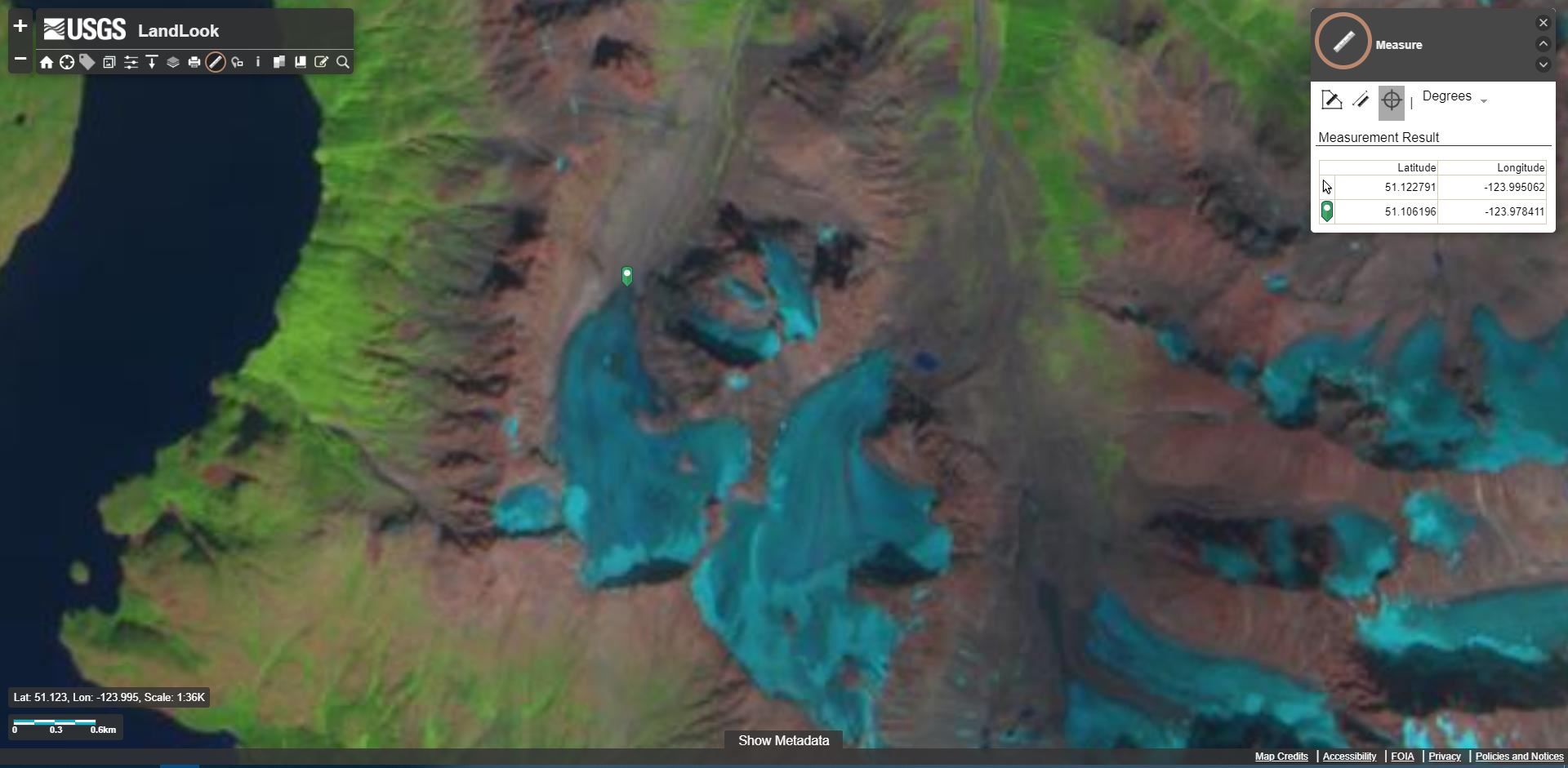
Step 3: Analyze the accumulation zone in the most recent satellite imagery (Figure EX2.4).
- Go to the Sentinel Playground for viewing recent satellite imagery and navigate to a large scale view of your glacier.
- View your chosen glacier by typing in the coordinates or name of your glacier or name of your glacier in the search pane (magnifying glass icon) and zoom in until the glacier fills a lot of your map area.
- In order to find the date of the best Sentinel 2 image capturing the most recent size and pattern of the accumulation zone, use the calendar at the top of the page. Inspect the summer and early fall images in order to find the year's true accumulation zone. This date coincides with the time of year when the size of the preserved snowpack from the previous winter will be at a minimum. Therefore, set the date range for your search to mid or late summer. For glaciers in low latitudes (southern and central BC or Alberta), someone would typically need to inspect from early August to late September. For glaciers in higher latitudes (Yukon, Nunavut and northern BC or Alberta) inspect from early July to Late August. Howerver, anomalous years do occur and one might need to look at later years.
- Once you have found the best image, use the menu on the left, and set the menu to Custom and drag the following Band onto the output fields R:12 G:8a B:4 . This band combination accentuates snow surfaces from ice as well as water.
- Press the Generate button. Copy the URL of this image (button on bottom) and download the image.
- Create a screen capture of the glacier and save it in a file named <8_Lastname_daymonthyear_Sentinel_2_image>.
- Add this file to your document as Figure EX2.4 (refer to Figure 22.7 for an example) and indicate the image source by adding the URL of your current view. Do this by using the Bookmarks button then Generate URL button.
- Write a caption in which you describe and discuss the following questions:
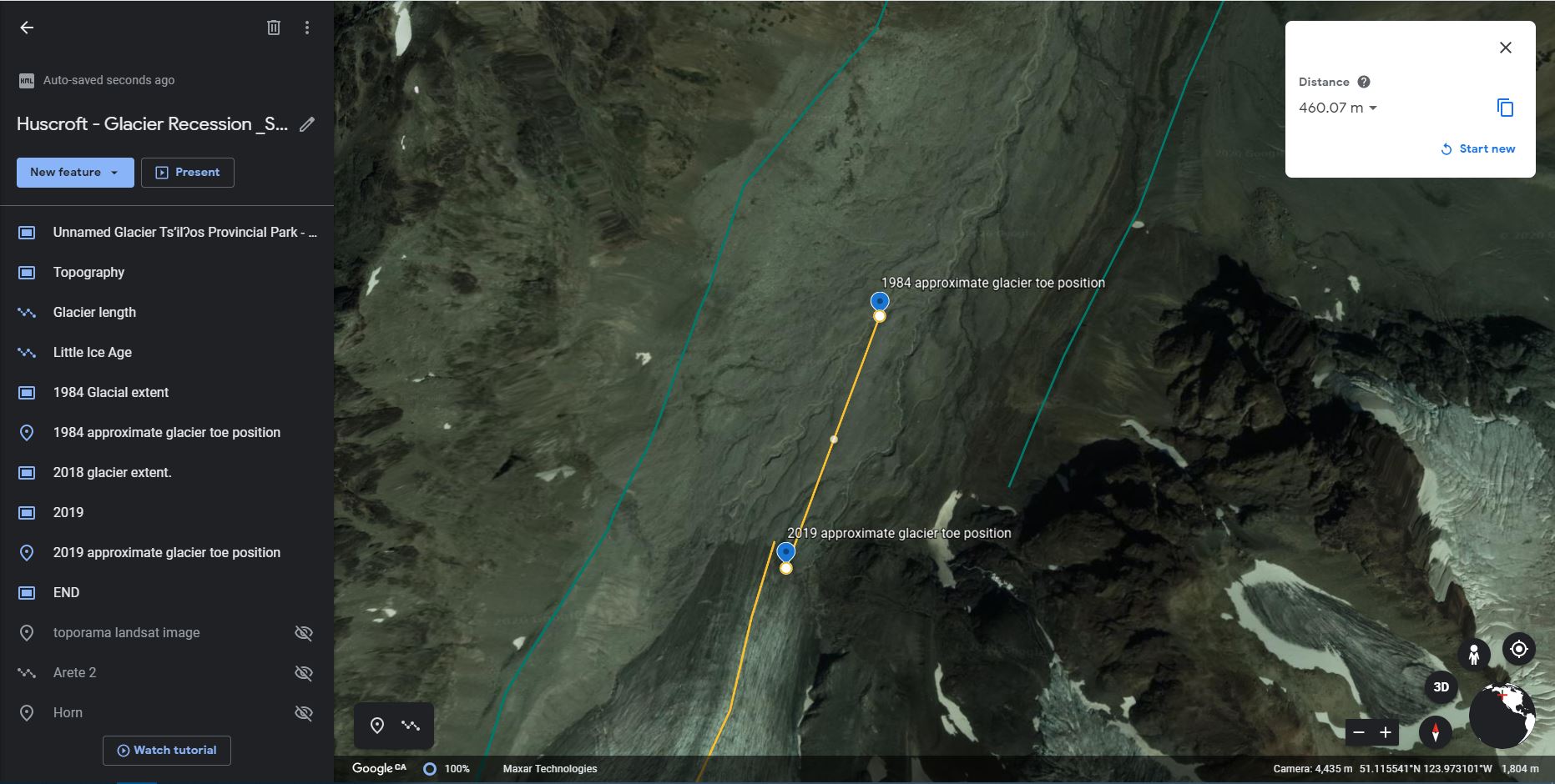
Step 4: Calculate the rate of change (Figure EX2.5).
- Using the coordinates recorded in the previous step, add a point to your Google Earth (Web) project called <Year approximate glacier toe position>. For example, 2024 approximate glacier toe position.
- Measure the distance between this location and the 1984 position and calculate the average rate of retreat or advance of the glacier. Take a screen capture of this measurement and save the measurement as <9_Lastname_glacier_position_measurement>. Add this image to your document as Figure EX2.5. An example is provided as Figure 22.8.
- Write a caption that includes the total measured retreat (or advance) distance over the period from your earliest photo until the most recent satellite imagery, and the average rate of retreat.
Step 5: Get curious and do a small scientific analysis of your own choosing.
- By exploring the tools and images available to you on the websites you have used so far in this lab, do an extra analysis of your own creation and add extra screen capture(s) as figure(s) that support your analysis as Figure EX2.6 (and additional if needed). Try to keep it as simple as possible. Be sure to state the question you are trying to answer in your analysis as well as your method. Possible analyses could involve:
- Doing an extra measurement.
- Accessing imagery from a different time and doing comparisons.
- Finding imagery on the The Atlas of Canada - Toporama website or the iMap BC website and comparing glacier toe positions.
Reflection Questions
- Which part of this activity did you like the most and why? Which did you like the least and why? In which section did you feel you learned the most about glaciers?
- In one paragraph, share your feelings about:
- Your discoveries in this lab in regard to the survival of your glacier.
- The fact that your classmates have probably come to similar conclusions with respect to other Canadian glaciers.
- How you felt being able to view historical images in order to come up with your own scientific conclusions about a glacier of your choice.
Report Submission
- Review your text for grammatical and spelling mistakes.
- Export your document to a PDF. Your PDF file needs to be a reasonable size (generally less than 5MB, but ask your lab instructor for details). In order to do this, you will need to reduce (compress) the file size of all of your images to between 150-100 ppi. Be sure to check that you have not compressed the images so much that you are not able to see them clearly on your monitor. For PC users, the compression can be done with MSWord by clicking on the image, choosing Picture Tools - Compress.
Submit as directed by your instructor.
Worksheets
Sample Student Assignment
References
GISGeography. (Last updated 2021, February 27). 5 free historical imagery viewers to leap back in the past. https://gisgeography.com/free-historical-imagery-viewers/
Pelto, M. S. (2010). Forecasting temperate alpine glacier survival from accumulation zone observations. The Cryosphere 4, 67–75. https://doi.org/10.5194/tc-4-67-2010
Media Attributions
- Video 22.1: Sacagawea Glacier, Wind River Range Wyoming Survival by Mauri Pelto is licensed under Standard YouTube License.
- Figure 22.1: Image from Google Earth. Used in accordance with Google Earth terms and conditions. Adapted by C. Huscroft.
- Figure 22.2: Image from The Atlas of Canada- Toporama. Used in accordance with Government of Canada non-commercial reproduction terms of use. Adapted by C. Huscroft.
- Figure 22.3: Image from Google Earth. Used in accordance with Google Earth terms and conditions. Adapted by C. Huscroft.
- Figure 22.4: Image from Google Earth. Used in accordance with Google Earth terms and conditions. Adapted by C. Huscroft.
- Figure 22.5: Google Earth Engine Timelapse – glacier from Google Earth. Used in accordance with Google Earth terms and conditions. Adapted by C. Huscroft.
- Figure 22.6: Image from Google Earth. Used in accordance with Google Earth terms and conditions. Adapted by C. Huscroft.
- Figure 22.7: Image from USGS LandLook is in the public domain.
- FIgure 22.8: Image from Google Earth. Used in accordance with Google Earth terms and conditions. Adapted by C. Huscroft.
