Lab 13: GPS Orienting
Saoirse MacKinnon and Craig Nichol
Geospatial information is important to anyone wanting to analyze the spatial configuration of Earth’s surface, including those features that are natural (e.g., rivers, lakes, mountains) or human-made (e.g., streets, buildings). Geospatial Information Science (GISC) is the discipline that deals with geospatial information. Geographic information systems (GIS) are software programs designed to work with geospatial data. Over the last two decades, GIS have become ever more powerful and widely used in day-to-day life. This exercise will allow you to become familiar with a couple of the most frequently used geospatial programs: Google Maps and Google Earth.
This lab provides experience in using Google Maps to navigate a route and record GPS coordinates, and using Google Earth (Web) to produce point location stops with photographs and add a path to outline the route taken on the produced tour.
Learning Objectives
After completion of this lab, you will be able to
- Use Google Maps to obtain coordinates for stops of interest (i.e., waypoints).
- Pin waypoints in Google Earth (Web) using the coordinates obtained with GPS.
- Import and attach photographs to Google Earth (Web) pins.
- Translate a walked route from Google Maps into Google Earth (Web).
- Exhibit a subject of interest as a virtual tour in Google Earth (Web).
Pre-Readings
In order to complete this lab, some background information in digital positioning systems, mapping with a smartphone, geographical information systems, and using Google Earth web is required.
Digital Positioning Systems
Locating yourself on Earth has become much simpler since the creation of digital positioning systems. The most well-known of these is the satellite-based Global Positioning System, more commonly known as GPS. The core of the GPS system is composed of dozens of satellites that orbit Earth at 20,000 km altitude. Each satellite has a precisely synchronized clock on board, and the satellites are constantly tracked so their precise position is known at any instant in time.
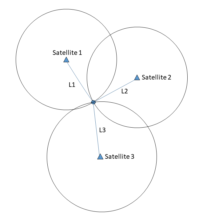
The satellites emit a time-coordinated signal that can be detected by a GPS receiver on Earth. Receivers track the signal from multiple satellites at once: 4 or more are needed for best accuracy. The timing of when that signal left the satellite, and the position of each satellite when the signal was sent is known and available to the receiver. The distance from each satellite to the receiver is calculated using the time offset between when the signal arrives from the each of the different satellites, and the velocity of those signals in the atmosphere. A spherical surface of radius L can be defined that includes all points in space that are at the same distance away from that satellite. (This is why having only one satellite would not be much use.) Knowing the distance between the ground-based receiver and multiple satellites allows you to calculate the location where all the spheres intersect, and this represents the receiver location (Figure 13.1).
The GPS system relies upon the receiver having a default model of the atmosphere in order to calculate distances. Variations in the properties of the atmosphere at any given moment cause slight errors in the calculations, but with multiple satellites, the location of the receiver can be determined to about 5 to 10 m accuracy. Greater accuracy can be achieved with high-quality receivers, but requires considerable post-processing of the data to account for atmospheric effects.
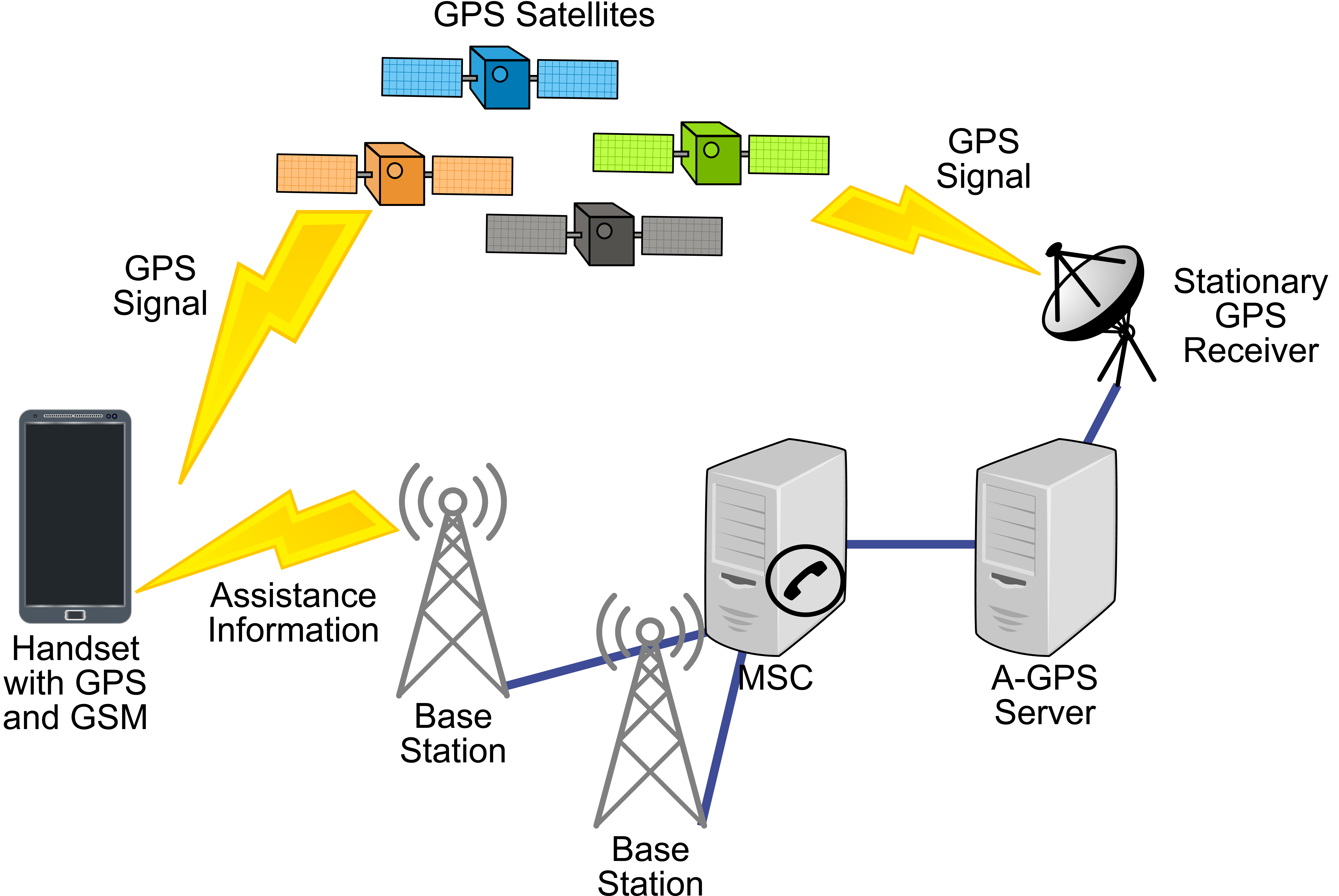
The accuracy of the basic satellite system was improved by deploying a number of permanent land-based receivers to provide wide area corrections. These base stations have exact coordinates that are fixed and precisely known (Figure 13.2).
The ground base stations determine their calculated coordinates based on GPS signals, and powerful comput
ers then determine the offset between the GPS calculated location and the actual known location. The data are broadcast as corrections to nearby receivers in real time (i.e., almost instantaneously). For example, if the GPS signal at the base station determines coordinates that put it 1 m to the east of its known location, then the GPS system distributes a message to all local receivers that any coordinates being calculated right now should be corrected by 1 m to the west before being shown to the user. This compensates automatically for atmospheric distortions of the satellite communication signals due to clouds, inversions, and storms, for example.
There are around 50 base stations in North America, which means a user might be 100s of kilometers or more from the nearest station. The corrections are more accurate close to the station, but a typical hand-held receiver may achieve ~1m accuracy with such wide area correction, if available.
The most accurate GPS systems are known as differential GPS systems. These use a ground receiver located within at most a few kilometers of the high-accuracy mobile receiver. Atmospheric corrections are made in real time for local conditions close to the receiver that allows locations to be obtained to within centimeters or sometimes better.
Mapping with a Smartphone
Your smartphone or tablet typically contains a GPS receiver that is likely of a slightly lower quality than a dedicated handheld GPS receiver. Cellular devices also use other means to locate themselves, such as pings to nearby cellular towers installed by the telecommunications provider. The towers transmit at known powers, and each cellular device has a known power of transmission. The variation in signal strength between the device and the towers can be used to estimate the distance from each tower.
Similar to the GPS satellites, the estimated distance from each cell tower defines a sphere around the tower, and the intersection of those spheres locates the transmitting device via triangulation. In some cases, the time of travel of signals from a phone to different towers can also be used to estimate distances in the same way as GPS data.
There can be complications, however. Buildings in urban areas and other parts of the built environment can block, reflect or alter signals. In cities, cell towers may be able to locate a cellular device to within 50 m from signal strength. Outside of cities, multiple towers may be far apart and accuracy is lower, or only one tower may be available, and no detailed location can be determined other than an estimated distance range from the tower.
Smartphone Location Settings
You will be mapping locations in the field during the lab using mapping software built into your mobile device. Make sure that you have determined how to turn on and off your device’s location settings. In Android, it is under your main device settings. In some versions Location is there as a setting. In other versions, you may have to look under Biometric and Security. You may also be able to swipe down from the top of your screen to access a quick link to turn location services on and off. On Apple devices, Location Services is found in Settings → Privacy. Typically, when you turn on any mapping app such as Google Maps, you will be prompted to turn on your location service, in which case you won’t need to search in your settings to turn on your GPS.
Software
Spatial mapping software is a common feature of most smartphones for providing directions. The two most commonly used programs for navigating are Google Maps and Apple Maps. Google Maps operates on all smartphone operating systems and therefore will be the software package we use for the lab.
Prior to the lab, download the Google Maps app to your smart device. Take some time to experiment with Google Maps before the start of the lab. There are a wide range of introductory Google Maps tutorials on the web to help you practice the following:
- Opening Google Maps in map view (the default view).
- Typing in an address and asking for walking (pedestrian symbol) and driving (car symbol) directions from where you are.
- Typing in a feature and asking for directions on public transit from where you are. Look for the bus icon. Which bus should you take? How long does it take?
- Searching for a category of things. For example, search Grocery Store.
- Switching to satellite view and back to map view. Take some time to scroll around where you live using the satellite view. Can you find any forested areas?
- Dropping a pin at a location. On a smartphone, this involves pressing and holding on a chosen location.
We will use this last skill in the lab, and you can experiment with this prior to the lab. To mark a point:
- Zoom in to the location where you wish to mark a point. Do this by pinching two fingers in to zoom out, and apart to zoom in.
- Place your finger on the location you wish to mark, and hold it until a Pin is dropped on that location.
- The latitude and longitude of the location in decimal degrees will be displayed in the top menu bar. These can be written down.
- The point can be shared with yourself by clicking on the share icon. You can email or text the point in order to keep it.
- You can click on Label, choose a name for the point and then save the point to your device.
Geographical Information Systems (GIS)
Cartographers are routinely faced with trying to reconcile different datums, spheroids, old maps, new maps, GPS data, and survey data, all using hand calculations. Even with powerful computers, the task is complex and arduous. The evolution of Geographic Information Systems (GIS) has hugely simplified such routine tasks as coordinate transformations and has opened up new ways of mapping features and processes on Earth’s surface.
GIS comprise both the hardware and software that are fundamental to the mapping enterprise, but it is increasingly common for people to use GIS generically in reference to the class of computer program that are available for use. For example, Google Earth, ARC GIS, and QGIS are three of the most commonly used GIS programs, but there are several others (e.g., GRASS).
These systems are capable of storing spatial coordinates (in all their varying forms and coordinate systems) as well as any attributes associated with that location. For example, when taking a hike in the woods, you may come across an earthen mound that you suspect contains artifacts of interest to First Nations. Rather than disturb the site, you take a waypoint (i.e. the coordinates of the site) and enter a note describing the feature as an earthen mound possibly containing artifacts then upload a photo. The note and photo are attributes rather than coordinates.
How GIS Store Spatial Information
GIS systems are based on storing spatial data using three fundamental data types: points, lines, and polygons.
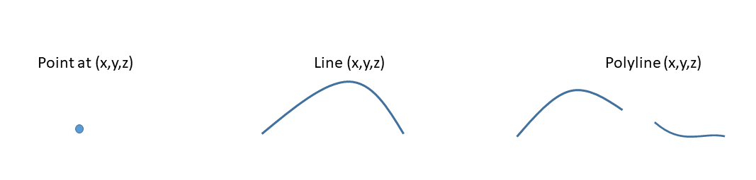
A point is a single location in space defined by a set of coordinates (Figure 13.3, left). We will be using latitude and longitude expressed in decimal degrees, and elevation (in metres). Each point can have attributes that are associated with that single point and stored in a data table.
A line is formed by connecting a series of points (Figure 13.3. middle). The line that connects the points can be straight line segments or interpolated curves. The attributes are associated with all locations along the line, not just the points. The term polyline is often used because the line does not necessarily have to be continuous (Figure 13.3, right). Data stored in the table of attributes can be in multiple formats: integers, real numbers, text, images, etc.
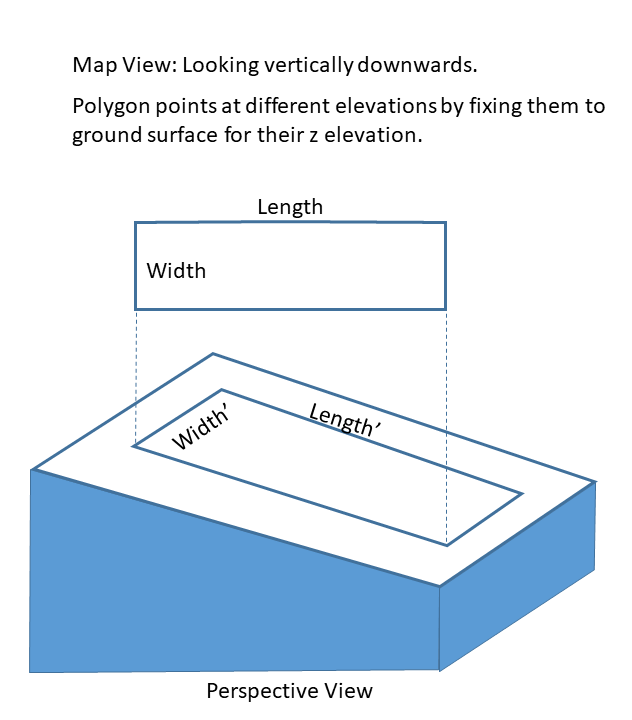
A polygon is a closed shape formed by connecting a series of points. A polygon can define a two-dimensional shape where the shape is defined in x and y coordinates only (Figure 13.4). If the world was flat, then the length and width in map view (looking down from above) would be the same as the length and width on the ground.
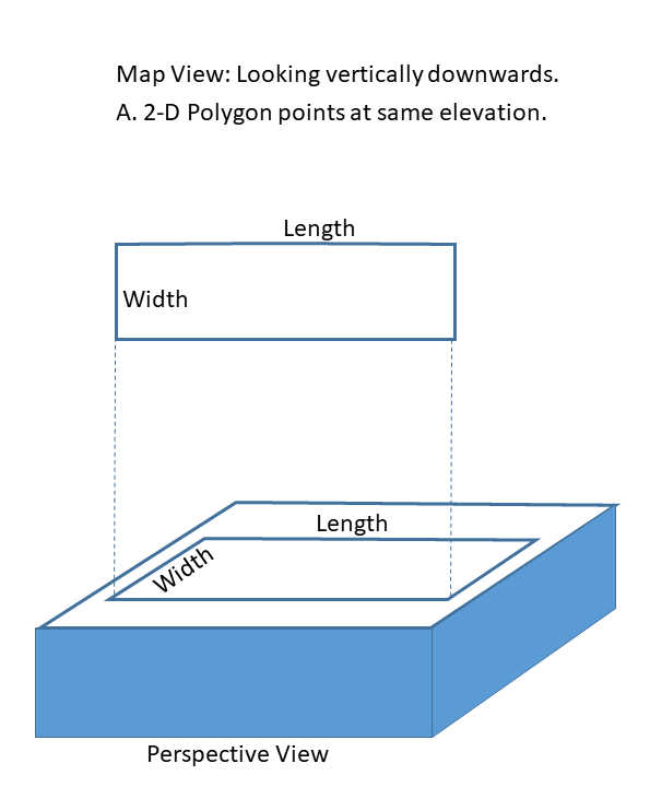
A three-dimensional polygon requires that x (longitude), y (latitude), and z (elevation) coordinates be entered for each point. One way to do this is to define coordinates in x and y only, and then let the geographic information system assign the elevation coordinate to be equal to the ground surface elevation that it has stored in some other way (Figure 13.5). This is a common way to make polygons in Google Earth. In the example shown, the size of the rectangular polygon is defined first in x and y only in a Map View, and it has a length and width in this example. The length and width on the ground (denoted length’ (pronounced length prime) and width’ (pronounced width prime)) will be different because the polygon has a z dimension to it. When you measure the area of the polygon, it is important to know which area you need: map-view 2D area, or on-the-ground 3D area.
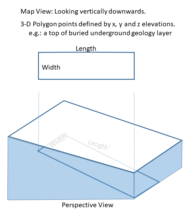
Three-dimensional polygons can also be created by assigning x, y, and z coordinates to the polygon right from the start (Figure 13.6). The GIS system starts with the full 3D data seen in the perspective view (length’, width’). It can project this onto the map view to determine what the polygon shape looks like if you are looking directly downwards. It is important to understand what area is being calculated when you request an area value: the area of the polygon in map view (length multiplied by width), or the actual area defined on the ground (length’ multiplied by width’), which could be larger depending on topography.
Using Google Earth (Web)
Like Google Maps, Google Earth was created to be very user friendly. It does not require specialized knowledge, and basic mapping functions are fairly intuitive. However, both programs have very sophisticated GIS capabilities behind them that can be used in ways similar to QGIS or ARCGIS.
There is a traditional desktop version of the program that can be downloaded and installed on your computer, but we will be using the online version: Google Earth (Web). This does not require you to download anything; you simply need to have internet access on your computer. Although it is now possible to run the web version of Google Earth in most internet browsers, Google Chrome is the recommended browser.
Refer to Video 13.1 for a thorough, but slightly outdated, tutorial that covers all of the basic functions of Google Earth (Web).
Video 13.1. Basic functions of Google Earth (Web).
It is likely easiest to open Google Earth in Google Chrome on a computer, but then watch the video on your mobile device so you can follow along. Alternatively, a large monitor or dual monitors may allow you to split the screen and have both the video and a Google Earth window open at the same time.
Make sure you are familiar with:
- Zooming in and out using the mouse wheel or the on-screen sliders.
- Panning using either grab and move with the mouse, or the on-screen pan tool.
- Tilting the view using the on-screen view.
- Determining the coordinates of the point your mouse is pointing to. To do this, look along the bottom of the screen.
- Measuring the elevation of the ground.
- Determining the elevation of your eye height.
- Turning on and off items in the places or layers menus to the left.
The lab exercises will require you to enter point coordinates as pins, add a path, and import and attach photographs to the pins.
Lab Exercises
In this lab, you will be producing a local photograph tour of a subject of interest to you. This will involve going outside near where you live (or elsewhere) and taking photographs and GPS coordinates of a number of spots that demonstrate your subject of interest. Then, you will upload the coordinates and photographs as points in Google Earth (Web). Lastly, you will add a path between points to reproduce the route for your tour. The lab should take 2-3 hours to complete, including approximately 1 hour outside.
The lab requires a smartphone (Android, iOS, Windows) with a data plan and Google Maps installed. If you do not have a smartphone and/or you do not have an active data plan, contact your instructor to arrange for an appropriate modification to the lab exercises based on what technology you do have access to.
EX1: Field Collection of Coordinates and Photographs
Safety note: do NOT complete this exercise until receiving a safety briefing and filing the proper paperwork (if applicable). Your first responsibility when arriving at a site is to ascertain whether or not the terrain is safe to traverse. If not, find a new location.
Step 1: Choose a subject of interest.
This lab is an opportunity to show off a subject that interests you. The restrictions are that the subject has to be found outside, within walking distance of where you live (or within a reasonable travelling distance, if you are willing to travel), and there must be 5-10 points that can be taken at different spots as part of your subject of interest. The points cannot be too close (you cannot use 7 trees in a row) but must be close enough that you can reasonably walk between them.
The following lists some suggestions for points of interest. The suggestions are intended to help you come up with your own ideas, but they can be used if you cannot think of anything else.
- Parks and green spaces that are within walking distance (5+)
- Your favourite walking/hiking trail and points of attractions
- Good nature and/or bird watching sites in your local area
- Bus stops, coffee shops, or bookstores (5+ stops, a better option in cities)
- Different tree and/or plant species that can be found nearby
- Best places to eat that are in your local area (better option in cities)
Step 2: Do some online research (optional).
If you pick a subject of interest that you know little about, spend a bit of time researching it online before heading outside. After you have researched the subject a bit, open Google Maps on your computer or smartphone before wandering outside, and look for your address and potential stop points.
If you have chosen something you are already familiar with (i.e., you are looking at birds in your community and you bird watch daily), this step can be skipped.
Step 3: Prepare your field notes.
Open the Field Notes Template in Worksheets. The provided template includes a table for recording your stop descriptions and point coordinates, and a space for a field sketch of your route. This page can either be printed out, or reproduced on paper you have on hand. Make sure you have this ready to go before going outside.
Step 4: Locate and go to your first stop. Collect coordinates, notes, and a photograph.
Once you are at your first stop, open Google Maps on your mobile device. (Make sure the data option is enabled if you don’t have this set as the default). You should see the location that you are at. As a reminder, mark a point at your current location:
- Zoom in to the location where you wish to mark a point. Do this by pinching two fingers in to zoom out, and apart to zoom in.
- Place your finger on the location you wish to mark, and hold it until a Pin is dropped on that location.
- The latitude and longitude of the location in decimal degrees will be displayed in the top menu bar. Write this down on your field notes.
- The point can be shared with yourself by clicking on the share icon. You can email, or text the point in order to keep it.
- Click on Label and choose a name for the point, and then save it to your device.
Record a description of your point and the latitude and longitude on your field notes. Then take a photograph of the subject of interest at this stop in landscape orientation. It is recommended that you take multiple photographs so you can select the best one later.
Step 5: Repeat Step 3 for the remainder of your stops.
Go to the second stop and collect coordinates and a photograph, then go the third stop and collect coordinates and a photograph, and so on. You need to have a minimum of 5 stops (a maximum of 10), and they need to be within a reasonable walking distance of each other, but not too close. If you can throw a ball between stops, they are too close.
Step 6: At your final stop, produce your field sketch.
Produce a field sketch of your route, including all of the stops. Since you have pinned your stops on Google Maps, you can zoom out and see them all at once. This will help with the general shape of your route, and relative distances between each stop. Your field sketch should also include a point of reference. A good point of reference is something that would show up on Google Maps or Google Earth if searched for, like a named school, library, or park. Your field sketch must be completed outside, and you are not permitted to reproduce it once inside. An example of a field sketch is provided in Lab 01 Figure 1.3.
Before leaving the field, take the following two photos:
- A close-up of your field sketch.
- A selfie of you and your field sketch in front of your final stop of interest.
Step 7: Return home.
Upload the photos of your stops and your field sketch to your computer and save to a known location. Submit the field sketch according to instructions provided by your instructor.
EX2: Producing Your Virtual Field Trip in Google Earth
Step 1: Set up Google Earth (Web).
Even if you are familiar with Google Earth – do NOT skip this step.
Open Google Earth (Web) in your internet browser (Google Chrome is recommended) and click Launch Earth in the top right corner.
Click the three horizontal lines on the top of the left hand menu to open the primary Google Earth menu. Click Settings to open the settings menu. Scroll down and make sure Units of measurement is set to Meters and kilometers. Change to this setting if it is not. Then, change Latitude/Longitude formatting to Decimal. Click Save.
We now have Google Earth (Web) set up the way we wish and are ready to enter data.
Step 2: Create your stops as points (placemarks) and upload photographs and descriptions.
If you have not done so yet, email yourself the photographs from your field walk-around and save them on your computer. Make sure to label the photographs so you can attach them to the correct stop numbers.
In Google Earth, the fifth button from the top on the left hand menu looks like a pin over top of a square. Click this icon and a dialog window will pop up to Make a new project. Click Create and then Create KML file. If prompted with a pop up asking if you allow Google to save to your computer, you need to allow it.
Click the pencil icon and enter Lab 13 <your name> as your project name, then enter a short description about what your subject of interest is and the general location where you completed the project. Click Enter or click outside of this window to save.
Click New feature and then click Add placemark. You can loosely point to your first stop, or you can randomly select a location for now. Title this place Stop 1: <stop title> and make sure you are adding it to your Lab 13 <your name> project. Then click Edit place and a window will pop up that will allow you input your photograph, a description, and the decimal degrees coordinates your recorded from Google Maps:
- Click the icon that looks like a camera with a + on it. Drag the photograph for stop one in to the drop box (or click Select a file from your device). Your image should now appear in the edit place window. Note: you may need to sign in to a Google account in order to have this file upload option (without signing in, you may only see three options: Google Image Search, Video search, and URL). If you do not have, and do not want to create, a Google account, discuss with your instructor an alternate means of submitting these photographs.
- In the info box (text box underneath Title), type Coordinates determined from Google Maps using an <your device> and a short description of why you chose this location. Leave the Info box as Small info box (the default setting once you have typed anything into the info box).
- In Placemark, click Show Advanced Options. Replace Latitude and Longitude with the coordinates you obtained from Google Maps. Click outside of the window and your placemark should move to your entered coordinates.
- Leave Grounding as Clamp to Ground.
- Under Set view manually, click Reset to defaults. Click the back arrow at the top left of this window to return to your project.
Your placemark for Stop 1: <stop title> will now be listed in your project, and you can go back in to look at or edit anything by selecting it and clicking the pencil icon.
Repeat this with all remaining stops. Your number of placemarks should be equal to the number of stops you made along your route. Double-check this before proceeding.
Step 3: Add a path between your stops to show the route you took.
Zoom out and pan until you can see all of your pushpins.
- In your project window, click New feature then Draw line or shape.
- Single left click at the tip of your Stop #1 placemark. This will set the first point of your route path.
- Then, place points along the path you walked until you reach Stop # 2. In other words, add enough points so that you have reasonably described the way you got to the field area. You will need to use judgement as to how many points you put in around curves. Place a point at the tip of your Stop #2 placemark.
- Continue placing points along the path you walked until you reach Stop #3. Place a point at the tip of your Stop #3 placemark. Continue doing this until you have reached and placed a point at the tip of your final pushpin.
- Click the final point a second time or press enter. Enter Route traversed as the Place title, make sure it is being saved in your Lab 13: <your name> project folder, then click save. Your path will now be listed in your project.
Step 4: Export your Google Earth output as a KML file.
Click the 3-dot icon in the top right hand corner of your project window, then click Export as KML file. This will download your project as a KML file. Navigate to your downloads folder on your computer to find the file.
Submit the KML file according to instructions provided by your instructor.
Reflection Questions
- Describe one thing you learned about your subject of interest by doing this lab in 2-3 sentences.
- If you zoom into your map with the path, you will likely notice that your pins do not perfectly align with where you know you were standing when you were outside. They are likely off by a few metres or more. Based on the pre-readings, what are some likely explanations for this lack of proper alignment?
- Knowing what you now know about Google Maps and Google Earth, what would you do differently if you were to do this lab again from the start? If you wouldn’t change anything, why did your approach work, and what expert advice would you give to another student working on this lab to help them succeed? Write 2-3 sentences.
- You have a friend coming to where you live for the first time, but you just came down with cold-like symptoms and need to self-isolate from them. You just finished this lab, so you decided to make them a Google Earth tour of the must visit spots where you live. Where would you suggest they go? And how would you produce it? Write a concise 3-5 sentence plan for making the tour.
Worksheets
Print this page out in advance of heading outside, or recreate it by hand on lined or blank paper that you have on hand. Once completed, these are your field notes and must be handed in. You must not rewrite these notes. You need to photograph or scan this page as it looked when you returned inside and include it in your submission for EX1.
- Lab 13 Field Notes Template [Word]
- Lab 13 Field Notes Template [ODT]
- Lab 13 Field Notes Template [PDF]
Media Attributions
- Figure 13.1: Image by C. Nichol is licensed under a CC BY-NC-SA 4 .0 licence.
- Figure 13.2: Image by Adlerweb (2017) [SVG] is in the public domain.
- Figure 13.3: Image by C. Nichol is licensed under a CC BY-NC-SA 4 .0 licence.
- Figure 13.4: Image by C. Nichol is licensed under a CC BY-NC-SA 4 .0 licence.
- Figure 13.5: Image by C. Nichol is licensed under a CC BY-NC-SA 4 .0 licence.
- Figure 13.6: Image by C. Nichol is licensed under a CC BY-NC-SA 4 .0 licence.
- Video 13.1: New ONLINE Google Earth: Web-Based Google Earth by Technology for Teachers and Students is licensed under a Standard YouTube License.
Image Descriptions
Figure 13.2. Schematic representation of the correction data provided to GPS receivers by GPS ground stations and servers.
A schematic example of how corrected GPS data is sent to GPS receivers by GPS ground stations and servers. GPS satellites orbiting the earth provide GPS signals to the ground. These are picked up by both handsets with GPS capability (GPS units, cellular phones, etc.), and stationary GPS receivers. The stationary GPS receiver communicates with a GPS server and base stations to correct the GPS data for real time local atmospheric conditions. The base station then communicates with the handheld GPS unit (if it has this capacity) to correct the GPS data that was provided directly from the GPS satellites. This can increase the accuracy of the GPS data from approximately one meter accuracy, to approximately one centimeter accuracy (sometime even more).

![Adlerweb (2017) [SVG]](https://commons.wikimedia.org/wiki/File:A-GPS.svg)