In this lab you will be doing a combination of field and office-based analyses of topographical slope. In the field, your technique will simulate a quick low-cost method of approximating slope, and your office-based analysis is typical of preliminary office-based investigations.

Slope is a measure of change in elevation over a known horizontal distance. Often it is used to describe the steepness of a landform surface. One might argue that slope is one of the most significant landscape metrics for geographers to evaluate.

Much of Earth’s surface is sloping, not flat, and as a consequence there are a range of hydrological and geotechnical processes that are activated by the difference in potential energy between one location and another. Potential energy is the energy available to for doing work. For example, an object that is lifted above Earth’s surface to height H can be moved downward a distance H by gravity. Slope processes bridge several scientific fields such as geomorphology, soil science, hydrology, and engineering.

In this lab you will gather your own field measurements at a location of your choosing, and learn the basics of taking high quality field notes to support your field measurements. Then you will input your field measurements into Google Earth (Web) to help calculate the slope you observed in the field. Finally, using a Geographic Information System (GIS), you will measure the gradient of a ski run at a resort of your choosing, plot the vertical profile and produce a short report summarizing your findings.

Pre-Readings

Why Is Slope Analysis Important to Geographers?

Important applications for slope analysis include describing landforms, watershed modelling, characterization of wildlife habitat, assessing slope stability and mass wasting hazards, classifying soil development, modelling wildfire risk, and assessing potential for land use development.

Recording Field Notes: General Guidance

In the field you must be very neat and organized in recording information. In professional settings, notebooks are used as evidence that you used proper procedures and conducted yourself professionally by collecting all the relevant information. Occasionally, field notes are entered into legal proceedings as evidence in support of proper professional processes. It is important to start early in one’s career with taking well formatted, complete, and proper notes. Field notes will be the only recorded evidence of what you saw and did in the field. There is a saying, “if it is not in your field notes, it never happened”. Moreover, human memories are surprisingly unreliable, and it will take only a matter of a few days before you have completely forgotten the details of what you did in the field. Field notes are invaluable in this regard.

In professional settings, erasing mistakes is regarded as tampering with field notes. As such, you may not erase mistakes or cover them with white-out. Instead, neatly cross out any incorrect measurements. You never know if or how your observations and measurements will be useful later.

Surrounding Information

In the field, you will be recording GPS position, vertical distance measurements, and photographic images. However, before you take these measurements, there are other important pieces of information to be recorded. Surrounding information is always included so that the measurements become meaningful to other colleagues, employees, or researchers that read your values. This surrounding information includes:

• Location (coordinates and verbal description of relative position to major landmarks nearby);
• Date & time;
• Participants (include who is in the field and their roles);
• Weather (as the weather will influence the quality of your observations, measurements, and notes); and
• A description of your overall goal for this field stop.

Photographs

You will be taking photographs for this assignment and they will need to be recorded (remember that professionally, if a record of taking a photo is not in your field notes, the picture was never taken). If you take a photo, the following details should be included:

1. File number (time of the photo is fine if you are using a cell phone).
2. Approximate compass direction the camera was pointing.
3. If there is an object for scale so that the viewer of the photograph can tell how large items are in the photo.
4. The subject of the photograph and any other information that is important for understanding why you took the picture.

Field Measurements of Elevation Change (Vertical Distance) Using Levelling

As previously mentioned, slope is a measure of change in elevation over a known horizontal distance. A sighting level is a device that allows a user to be able to aim their view along a true horizontal line. Using a sighting level and a known eye height to measure the change in vertical elevation between two points is an ancient technique that early civilizations used to design aqueduct and irrigation systems. It is also a modern technique used in professional settings, except that much more sophisticated digital surveying equipment is used.

We will be using GPS readings of horizontal position built into a smartphone to determine the change in horizontal position. So, you might wonder, why not use the GPS to determine the change in vertical distance too? Although handheld GPS-based measurements of horizontal position are typically accurate to within roughly 10 m, errors in vertical position are typically 2-3 times greater. Therefore, using a level to determine vertical distance can improve approximate measurements of slope over using hand-held GPS measurements alone.

As seen in Figure 16.1, if a level is used to sight a series of target locations on the ground (Point x₁ through to Point A’), and the level’s elevation above the ground (z) is known, the vertical distance (Δz) from A to A’ can be measured. The vertical distance (Δz) is also know as the rise of the slope from A to A’.

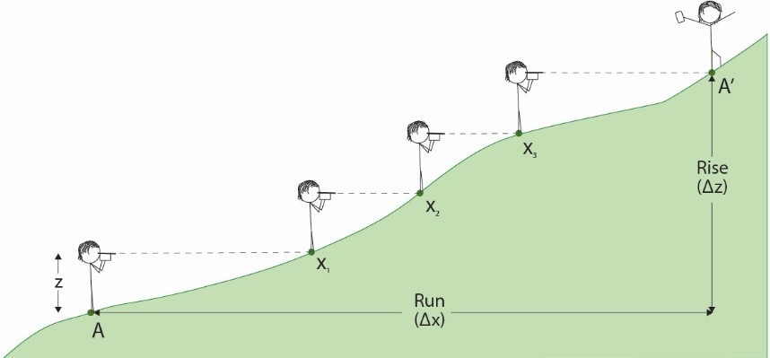
No matter the type of level that you use, there are several steps that are common to all levelling measurements of elevation change:

1. Measure the height between the ground and your instrument (z).
2. Start downhill and work your way uphill.
3. At the starting point A, sight along the edge of your level, as though you are aiming an arrow with precision toward the slope in order to locate your next sighting position (x₁). If you have a field partner, they can landmark the position of your target (x₁, x₂, etc.) for you.

Using a GPS to Record Horizontal Position

The Global Positioning System (GPS) uses the relative distance of a ground-based receiver to a constellation of satellites to triangulate and locate the receiver’s position on the Earth’s surface. Almost all cell phones are equipped with GPS-receiving technologies and they can be used in a fashion similar to a hand-held GPS receiver that is designed for terrestrial or marine navigation. Handheld systems are convenient to carry, give rapid readings with reasonable accuracy, and allow the user to record digital information about way points and paths.

As mentioned previously, handheld GPS-based measurements of horizontal position are typically accurate to within roughly 10 m under ideal conditions. However, errors in vertical position are typically 2-3 times greater. Ideal conditions include an open view of the sky without blockage due to buildings, bridges and trees so that the receiver can obtain signals from as many satellites as possible. A more in-depth description of GPS is described in the pre-readings to Lab 13 of this manual.

Calculating Slope Gradient

Your fieldwork and ski hill analyses will involve collecting data in order to analyze slope. In the first part of this lab you will obtain measurements of rise and run using a combination of levelling and GPS measurements. In the second part of the lab, you will extract this data from maps. After recording your field measurements, it is time to crunch some numbers. The gradient of a ground surface is calculated by the difference in elevation between two points on a slope (rise, Δz) divided by the horizontal distance between the two points (run, Δx). These two points are labelled as A and A’ on Figure 16.2, just as they are on Figure 16.1.

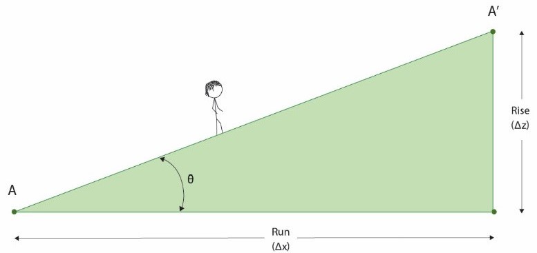
After obtaining the vertical elevation change (rise, Δz) and the horizontal distance (run, Δx) between two points, slope gradient can be calculated and expressed in three ways:

1. As a percent (%): the fraction (rise ÷ run) expressed as a percentage (Equation 16.1):

Equation 16.1

[latex]\text{Gradient} (\%) = \dfrac{\text{Rise, }\Delta z (m)}{\text{Run, }\Delta x (m)} \times 100\%[/latex]

2. As an angle, θ (degrees) (Equation 16.2):

Equation 16.2

[latex]\text{Gradient} (^{\circ}) = Tan^{-1} \left( \dfrac{\text{Rise, }\Delta z (m)}{\text{Run, }\Delta x (m)} \right)[/latex]

3. In elevation change per slope distance (m/km): the gradient expressed with different units used for rise and run, but with the run always reduced to one unit, commonly 1 km (Equation 16.3).

Equation 16.3

[latex]\text{Gradient} (m/km) = \dfrac{\text{Rise, }\Delta z (m)}{\text{Run, }\Delta x (km)}[/latex]

For example, let us assume that the elevation change we measured levelling between points A and A’ added up to 5 m, and the horizontal distance we measured between our GPS points using Google Earth is 200 m (Figure 16.3).

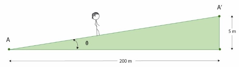
Using the equations presented above, we can express our slope gradient

1. As a percent (%) (Equation 16.1):

[latex]\text{Gradient} (\%) = \dfrac{\text{Rise, }\Delta z (m)}{\text{Run, }\Delta x (m)} \times 100\%[/latex]

[latex]\text{Gradientt} (\%) = \dfrac{5\text{ m}}{200\text{ m}} \times 100\% = 2.5\%[/latex]

2. As an angle, θ (degrees) (Equation 16.2):

[latex]\text{Gradient} (^{\circ}) = Tan^{-1} \left( \dfrac{\text{Rise, }\Delta z (m)}{\text{Run, }\Delta x (m)} \right)[/latex]

[latex]\text{Gradient} (^{\circ}) = Tan^{-1} \left( \dfrac{5\text{ m}}{200\text{ m}} \right) = 1.4^{\circ}[/latex]

3. In elevation change per slope distance (m/km) (Equation 16.3):

[latex]\text{Gradient} (m/km) = \dfrac{\text{Rise, }\Delta z (m)}{\text{Run, }\Delta x (km)}[/latex]

[latex]\text{Gradient} (m/km) = \dfrac{5\text{ m}}{\left( \dfrac{200\text{ m}}{1000\text{ m per km}} \right)} = 25\text{ m/km}[/latex]

Low gradient slopes are almost flat and have very little slope, whereas high gradient slopes have steep slopes.

Lab Exercises

This lab includes two exercises that result in creating an assignment to be handed in as a report in PDF format. The submitted report will include a series of required figures with captions.

Exercise 1 is partially field-based and will take approximately 3 hours to complete once you have found an appropriate field location (including report preparation but excluding travel time).

Exercise 2 is office-based. This exercise will take approximately 3 hours to complete. The length of time allocated to this exercise will depend on familiarity using Google My Maps, iMapBC, and Microsoft Excel.

Required materials:

• Tape measure or ruler.
• GPS equipped cell phone. Refer to your cell phone’s user guide. Almost all new phones are equipped with GPS capabilities. You may wish to choose an app set to record locations in decimal degrees.
• Material to construct a sighting level (see Appendix A).
• Pencil and field book or paper and a hard surface (clip board) to write on.
• Camera (cell phone is fine).

Required software:

• Google Earth (Web) – not mobile version.
• Spreadsheet software (Excel, Numbers, or Google Sheets).
• GPS App on your phone that preferably allows confirmation of communication with enough satellites. iPhones may use the compass tool if location services in your privacy settings is enabled. GPS Diagnostic is recommended and used by professionals, but costs a few dollars. Google Play offers GPS Satellites Viewer for free.
• Mobile levelling app for a phone/tablet or a level constructed from craft supplies (see Appendix A).
• iMap BC website (no user name required).

EX1: Determining Slope in the Field and Using Google Earth (Web)

Safety: Do not complete this exercise until receiving a safety briefing and completing the proper paperwork (if applicable) from your lab instructor. In addition, your first goal when you arrive at a site is to ascertain whether the terrain is safe.  

At Home Preparations

Step 1: Choose an Easily Accessible Slope.

Choose a slope that you can easily visit. This slope needs to be

• relatively steep with an elevation change at least twice your height,
• open (no obstructions to your view from the top to the bottom of the slope), and
• at least 100 m long.

Safe sidewalks and pedestrian overpasses with no intersections are appropriate, grassy hillsides as well as open and straight sections of trail are also good.

Step 2: Construct Your Level

Using the instructions in Appendix A, build your sighting level.

Step 3:  Measure Your Eye Height

Wearing the shoes that you will likely wear during fieldwork, measure the elevation of your eyes above the ground when looking level. If you do not have someone that can help you, or if you do not have a tape measure, stand beside a door frame and lightly mark the position of our eye height with a pencil by using your level to sight on the door frame. Use a ruler or tape measure to measure the elevation of your eyes.

Step 4:  Print or Copy Down the Field Notes Template

If you have access to a printer, print out the Field Notes Template in Worksheets to bring to the field. If you do not have access to a printer, copy the necessary information into your field notebook. This will be your Field Notes Worksheet.

Field Work

Step 1: Travel to the Field Site and Start Field Notes

After choosing a slope to measure, walk to the base of your slope. You will call this location Point A.

Record the surrounding information on your Field Notes Worksheet (participants, date, time, goal of fieldwork).

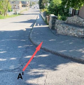
Step 2: Plan and Document Your Transect (Figure EX1.1)

Plan where you will start and approximately where you will end your slope measurement (location of Point A and Point A’). If you are using an open slope, it is best to travel directly up-slope (i.e., along the steepest trajectory) and not across the slope.

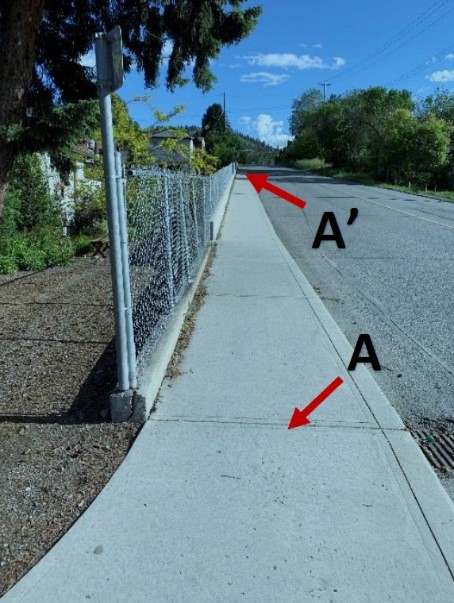
Document this plan by taking a photograph with your downhill start point (A) in the foreground and your approximate end point (A’) in the background. This will be Figure EX1.1 in your lab report (see the example in Figure 16.4). Record all pertinent photograph information (time or file number, direction of view, subject, verbal location description) about the photograph on your Field Notes Worksheet.

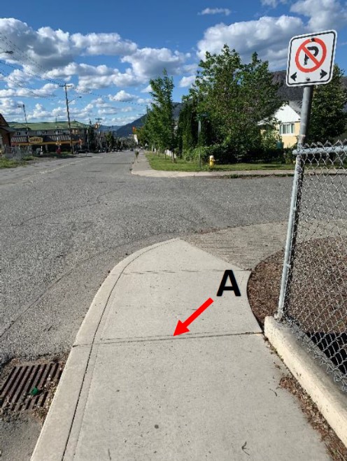
Step 3: Document Point A (Figure EX1.2)

While standing at Point A, record an accurate GPS reading (preferably in decimal degrees) by ensuring that you have at least 4 satellites. This may take a few minutes.

Include a verbal description of where Point A is located so that you will be able to tell if your location maps incorrectly into Google Earth.

Use a compass application on your phone to indicate the azimuth of your surveying. Azimuth refers to the compass direction expressed in degrees as a number between 0 and 360. Directions expressed as an azimuth do not include cardinal directions (north, south, east, west and their derivatives). For example, northwest has an azimuth of 305⁰.

Take an informative photograph of Point A. This photograph will be Figure EX1.2 of your report (see the example in Figure 16.5). Include the information you collect in this step in the figure caption. It may be helpful to annotate the photograph with the exact location of Point A with an arrow and label, although this can be done after the field with really good descriptions of where exactly you are placing the starting point (Point A). Don’t forget all the essential photograph information (time or file number, direction of view, subject, verbal location description).

Step 4: Level Up Towards Point A’

Standing at Point A (the base of your slope), use your level to landmark the position on the slope that is perfectly horizontal to your eye height (x₁ in Figure 16.1). Walk to your landmark (x₁) and repeat sighting to the next landmark position on the slope that is perfectly horizontal to your eye height (x₂).

Repeat and record the number of intermediate landmarks required to level up until your next sighting landmark is above your desired endpoint (i.e., where you would overshoot your desired endpoint if you continued). This last position at or above your desired endpoint will be your actual endpoint (Point A’).

Step 5: Document and Describe Point A’ (Figure EX1.3)

While still standing at Point A’, record an accurate GPS reading by ensuring that you have at least 4 satellites. This may take a few moments.

Include in your notes a verbal description of where Point A’ is located so that you will be able to tell if your measured location maps incorrectly into Google Earth.

Take an informative photograph of your actual endpoint Point A’. This photograph will be Figure EX1.3 of your report (see the example Figure 16.6). Include the information you collect in this step in the figure caption.

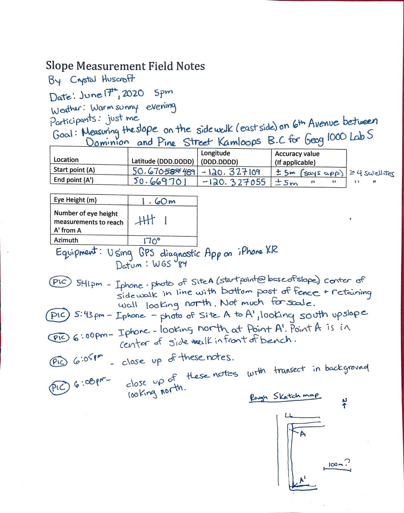
Step 6: Photograph Your Field Notes (Figure EX1.4)

Once you are done your field work, and before you leave the field, take a picture of your field notes in order to create a backup and include them in your report as Figure EX1.4 (see example Figure 16.7). Double-check by zooming into your photograph that your notes are clearly legible. Remember, you must not re-type or change your field notes in any way after you leave the field.

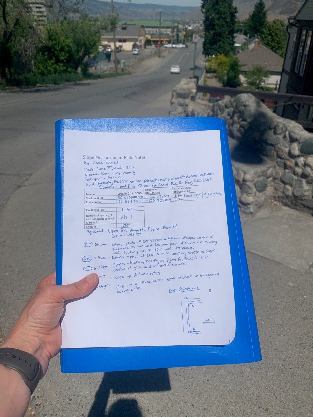
Step 7: Re-Photograph Your Field Notes with Transect in Background (Figure EX1.5) and Final Check

Retake a picture of your field notes with the location of your transect in the background as evidence of your work (see example Figure 16.8). Include in your lab report as Figure EX1.5. Before leaving the field, ensure that you are not missing any details in your notes and that you have taken all five of the required photographs.

Office Work

Step 1: Determine Horizontal Distance Using Google Earth (Figure EX1.6)

Once back from the field, open Google Earth (Web). Click on the Projects menu icon (fifth icon from top in the menu on the left of the screen). Then click New project and then Create KML file. Name your project <Lastname Firstname Student Number L16 EX1> by entering this into the box containing the text Untitled Project next to the pencil icon. Press the blue New Feature dropdown menu and choose Search to add place.

Input the recorded latitude and longitude of Point A and click the Add to project button once a placemark has been created.

Repeat the same steps to plot the recorded position of Point A’.

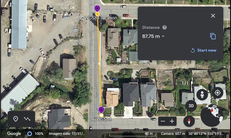
Once both Point A and A’ have been plotted, use the Measure tool (ruler icon at bottom of menu on left of screen) to determine the horizontal distance between Point A and Point A’. Create a screen capture of your horizontal measurement that includes the Google icon, camera, coordinates and elevation (see example Figure 16.9). This image will be Figure EX1.6 in your report.

Step 2: Calculate the Gradient

Calculate the vertical distance from Point A to Point A’ by multiplying your eye height by the number of sightings that you made in order to reach A’. Type out your answer and show your work in a clear table (see example Table 16.1). This will be Table EX1.1 in your report.

Calculate the gradient and express as a percentage, an angle, and as elevation change per km.

[latex]= \dfrac{\text{Rise, }\Delta z (m)}{\text{Run, }\Delta x (m)} \times 100\%[/latex]

Table 16.1. Example of Table EX1.1. Gradient Calculations

Calculation	Work (Including Intermediate Steps)	Calculation
Elevation change (field measured)	[latex]\small= \text{number of eye height measurements}\times\text{eye height}[/latex] [latex]= 6\times1.60 \text{ m}[/latex] [latex]= 9.6 \text{ m}[/latex]	9.6 m
Gradient (%)	[latex]= \dfrac{9.6\text{ m}}{92.15\text{ m}} \times 100\%[/latex] [latex]= 10.42\%[/latex]	10.42%
Gradient (°)	[latex]= Tan^{-1} \left( \dfrac{\text{Rise, }\Delta z (m)}{\text{Run, }\Delta x (m)} \right)[/latex] [latex]= Tan^{-1} \left( \dfrac{9.6\text{ m}}{92.15\text{ m}} \right)[/latex] [latex]=Tan^{-1}(0.104)[/latex] [latex]= 5.9^{\circ}[/latex]	5.9°
Gradient (m/km)	[latex]= \dfrac{\text{Rise, }\Delta z (m)}{\text{Run, }\Delta x (km)}[/latex] [latex]= \dfrac{9.6\text{ m}}{\left( \dfrac{92.15\text{ m}}{1000\text{ m per km}} \right)}[/latex] [latex]= \dfrac{9.6\text{ m}}{0.09215\text{ km}}[/latex] [latex]= 104\text{ m/km}[/latex]	104 m/km

Step 3: Assemble the EX1 Component of Your Lab Report

Use the list of figures and tables summarized in Table 16.2 to compile the first part of your report. Please ensure that your figures are large enough that they take up at least 75% of the area of a page. Do not forget to include descriptive captions for your figures, and to annotate the photos you use to create figures EX1.1 – EX1.3. Use your field notes to write the site descriptions.

Table 16.2. List of Figures and Tables from Exercise 1 to Include in Your Lab Report. Figure descriptions and example figures included.​Use this table as a checklist to make sure you have all of the necessary elements in your report.

Item	Description	Caption (Attribution)
Figure EX1.1	Photograph of entire slope used in Exercise 1, include direction and locations of A and A’	See example Figure 16.4 (Photograph Attribution)
Figure EX1.2	Photograph of Point A location	See example Figure 16.5 (Photograph Attribution)
Figure EX1.3	Photograph of Point A’	See example Figure 16.6 (Photograph Attribution)
Figure EX1.4	Field notes	See example Figure 16.7 (Photograph Attribution)
Figure EX1.5	Field notes with transect in background	See example Figure 16.8 (Photograph Attribution)
Figure EX1.6	Google Earth horizontal distance measurement	See example Figure 16.9 (Image Source – Screen capture must include Google logo and third-party data providers)
Table EX1.1	Include elevation change (field measurement) and gradient calculations in %, degrees, and m/km.	See example Table 16.1

EX2: Create a Slope Profile of a Ski Run at a Ski Hill in British Columbia

Step 1: Choose a Ski Run

Open Google My Maps. Click Create a new map. Using the search function on the left of your screen, visit a ski hill (resort) in British Columbia. The BC Ski Map contains more information about BC ski resorts. Zoom into the ski hill until all the lifts and runs are visible on the map. Select one ski run to use in this exercise.

It is recommended that you select a ski run below treeline which is easily traceable on satellite imagery. Ski runs should be longer in length, as short ski runs have few slope breaks. The ski runs at some smaller ski resorts may not be available on Google My Maps.

Step 2: Outline the Ski Run Using Google My Maps (Figure EX2.1)

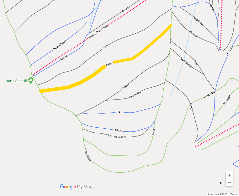
Select Add layer and draw a thick yellow line over the ski run selected (see example Figure 16.10). Include a screen capture of the run with the name visible in this exercise. Add marker adjacent to the bottom of the ski run and record the latitude and longitude of this location in decimal degrees. Share the Layer and copy the link to include in the Figure EX2.1 caption. Your caption should also include a description including the ski hill name and coordinates.

Step 3: Draw and Describe the Profile of the Ski Run Using iMapBC (Figure EX2.2)

Open iMapBC and launch application (Launch iMapBC). Select the option that does not require a username. Change the base map from Roads to Imagery. The icon is located in the bottom-left of the screen. The ski hill lifts and runs are not drawn in iMapBC, but they are visible as clear-cut areas in the imagery.

Find your ski run. Using the Lat/Long function in the tool bar, zoom to the run. To input Lat/Long, convert the units from decimal degrees to degrees, minutes, and seconds. Use the National Geodetic Survey Coordinate Conversion and Transformation Tool to convert, or consult the pre-reading Lab 14 Degree Conversions for instructions on how to do this by hand. Input the Lat/Long in degrees, minutes, and seconds to zoom into the ski run in iMapBC.

Add Provincial Layers on the Go to Data Sources tab. Search layer catalog for Contours – (1:20,000) (Base Maps – Contours – Contours – (1:20,000)).

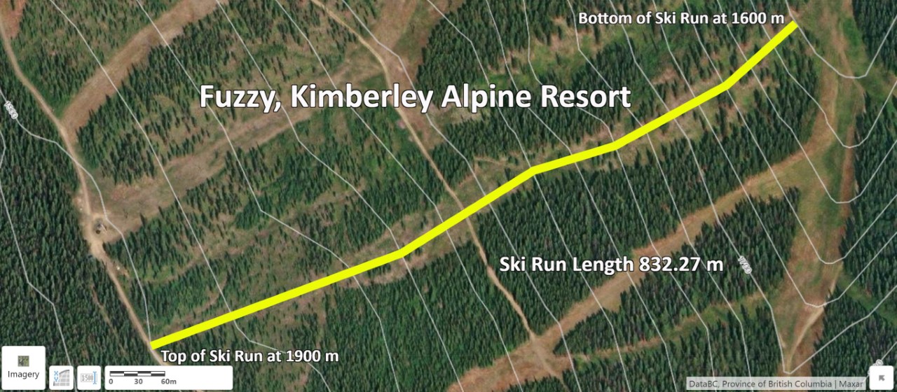
Create Figure EX2.2 for your report by drawing the ski run using the tools on the Sketch tab. Using the Edit tool, change the Styles of the line to change the colour and pattern of the line. Using the Identify tool on the Home tab, find the maximum and minimum elevation of the ski run. Using the Distance tool on the Sketch tab, measure the length of the ski run. Add Text to the map on the Sketch tab, including the name of the run, the run length (e.g., Run = 832.3 m), and the maximum and minimum elevation (see example Figure 16.11). Take a screenshot of the image.

Step 4: Describe the Natural Breaks in Slope for the Ski Run (Figure EX2.3 and Table EX2.1)

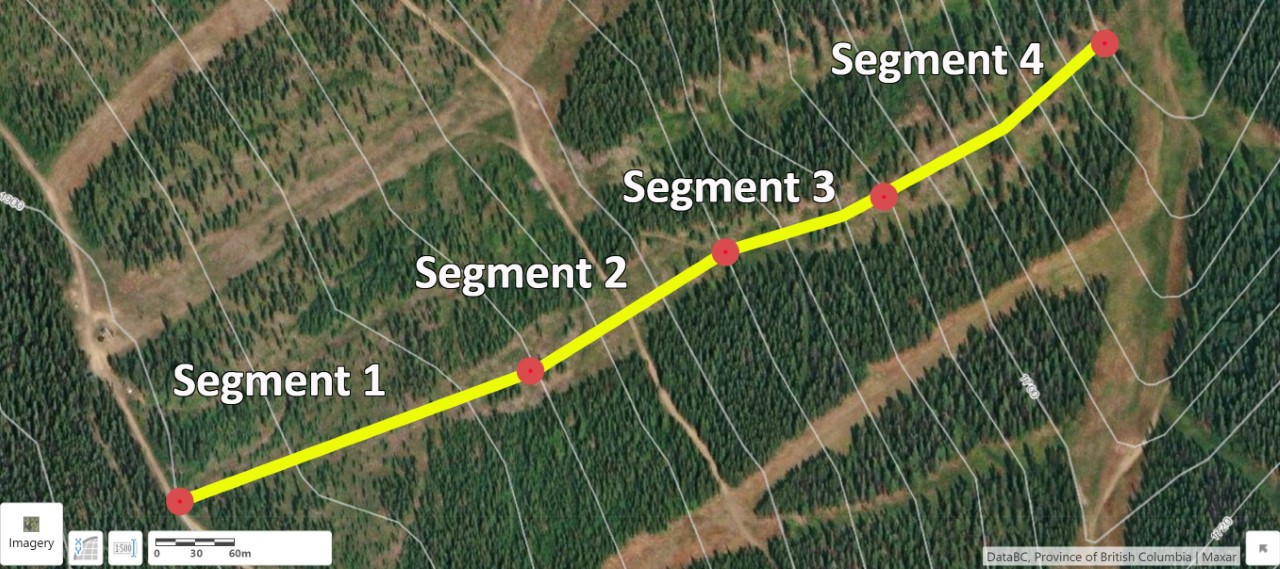
By inspecting changes in the spacing of contour lines along the path of the run, divide the ski run into 4 segments at natural breaks in slope. Breaks in slope indicate a change in physical continuity in the slope profile. Segments of your ski run may be steeper (more linear distance between contour lines closer together) than other sections.

Position your breaks in slope where your path (the ski run) crosses a contour line. Measure the horizontal distance between each slope break segment and record the elevation. This will be Figure EX2.3 in your report. Figure 16.12 is an example outlining four slope break segments selected for the Fuzzy ski run.

Create Table EX2.1 in your report to include the measurements you collected. An example is provided as Table 16.3.

Table 16.3. Example of Table EX2.1. Data Collected for Four Natural Slope Breaks Along the Ski Run Fuzzy at Kimberley Alpine Resort

Break in Slope Segments	Ski Run Distance for each break in slope segment (m)	Cumulative Ski Run Length (m)	Elevation Change for each break in slope segment (m)	Elevation at each break in slope (m)
Top of Ski Run (Segment 1)	–	0	–	1900
Bottom of segment 1	242.5	242.5	40	1860
Bottom of segment 2	237.2	479.7	80	1780
Bottom of segment 3	139.3	619	60	1720
Bottom of segment 4	213.3	832.3	120	1600
Total	832.3	–	300	–

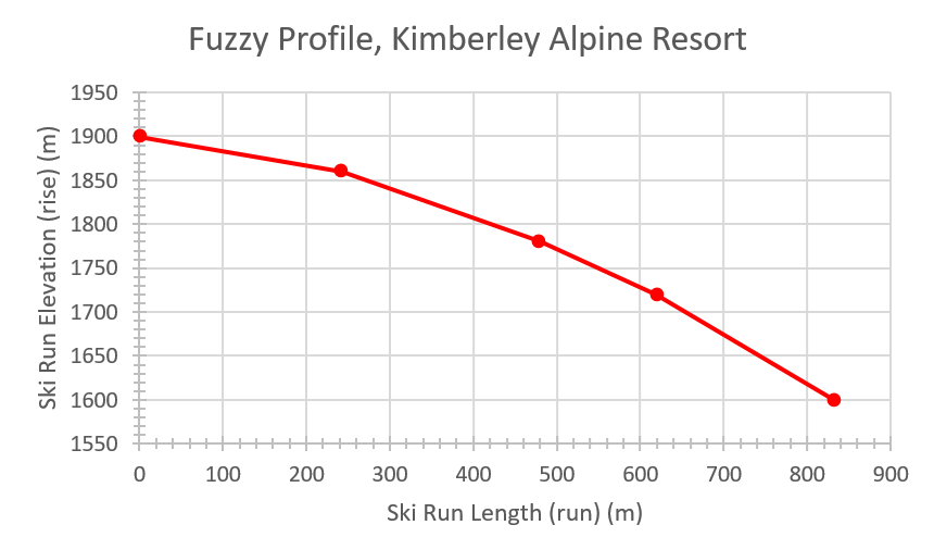
Step 5: Create a Profile in Microsoft Excel (Figure EX2.4)

Open Microsoft Excel and enter the data in columns similar to Table EX2.1 (Table 16.3). Figure EX2.4 in your report will be a profile of the slope using a Scatter (x.y) Chart (see example Figure 16.13, Example Figure 16.13 [Excel]).

Adjust the maximum and minimum values displayed on the ski run elevation axis (y) to optimize the range of elevation in the profile. For example, the y axis in Figure 16.13 ranges from 1550 m to 1950 m. Microsoft Excel will default the axis to start at 0 m.

Step 6: Calculate Gradient Using Microsoft Excel

Calculate the slope gradient in Excel using the three calculations provided in Calculating Slope Gradient. Calculating gradient in degrees in Excel requires the use of the =ATAN function. The complete Excel expression is =(ATAN(rise/run)*(180/PI())). ATAN is an abbreviation for arctan, which is denoted tan^-1. PI() is the notation for π in Excel.

Calculate the average gradient for each segment and include in Table EX2.2. An example is provided as Table 16.4.

Table 16.4. Example Table EX2.2. Gradient Calculations for the Ski Run Fuzzy at Kimberley Alpine Resort

Slope Segment	Gradient (%)	Gradient (°)	Gradient (m/km)
1	16.5	9.4	165.0
2	33.7	18.6	337.3
3	43.1	23.3	430.7
4	56.3	29.4	562.6
Average	37.4	20.2	373.9

Step 7: Assemble EX2 Component of Your Lab Report

Open the Word document created in EX1. Add EX2 and include Figures EX2.1 to EX2.4 and Tables EX2.1 and EX2.2 with detailed captions for each. Table 16.5 provides a checklist.

Table 16.5. List of Figures and Tables from EX2 to Include in Your Lab Report. Figure descriptions and example figures included. Use this table as a checklist to make sure you have all of the necessary elements in your report.

Item	Description	Caption (Attribution)
Figure EX2.1	Google My Maps screen capture of the ski run.	See example Figure 16.10 (Image Source – Google My Maps Attribution).
Figure EX2.2	iMapBC screen capture of the ski run including the name of the run, 20 m contour lines, maximum and minimum elevations, and run length.	See example Figure 16.11 (Image Source – iMapBC Attribution).
Figure EX2.3	iMapBC screen capture of the 4 natural slope breaks you used for your profile.	See example Figure 16.12 (Image Source – iMapBC Attribution).
Table EX2.1	Data collected for the 4 natural slope breaks you used for your profile.	See example Table 16.3.
Figure EX2.4	Profile of your ski run created in Microsoft Excel.	See example Figure 16.13.
Table EX2.2	Gradient calculations completed in Microsoft Excel for your ski run, including average slope.	See example Table 16.4.

Worksheets

Back to Lab Exercises

Field Notes Template

• Lab 16 Field Notes Template [Word]
• Lab 16 Field Notes Template [ODT]
• Lab 16 Field Notes Template [PDF]

Supporting Material

Appendix A: How to Build a Level

Back to Lab Exercises

This appendix describes two options for building a level. Choose the one that works for you:

1. Using an app on your cell phone;
2. Using a protractor template and craft supplies.

Option 1: Building a level using an app on your cell phone

Materials:

• Smart phone (recent model with accelerometer)
• Levelling app
  • iOS devices can use the Measure app installed by default on your phone. Just press level (bottom of screen).
  • Android phone users may want to try AR Measure.
• An 8.5”x11” piece of scrap paper rolled into a tube approximately the diameter of a straw
• Tape

Instructions:

Tape the paper tube along the long edge of your smartphone, while making sure that buttons do not get in the way of the tube being absolutely parallel with the long edge of your phone.

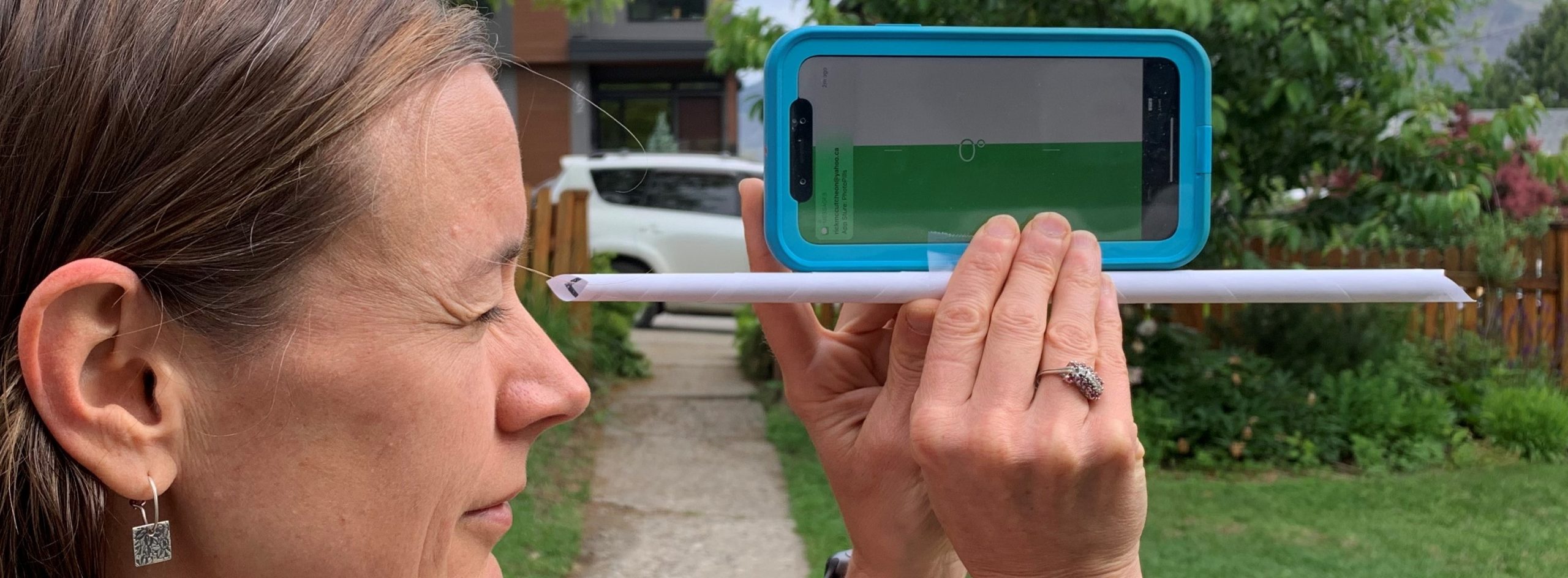
Using your paper tube, sight along the long edge of your phone as in Figure 16.14.

Option 2: Constructing your own level

Materials:

• Cardboard
• Protractor template (see Appendix B)
• 50 cm of thin string or sewing thread
• Stapler or tape
• A weight (such as a bag of coins)
• Scissors
• Paper glue
• Tape
• An 8.5”x11” piece of scrap paper rolled to the diameter of a straw and taped

 Instructions:

1. Print out and glue the protractor template (see Appendix B) to a piece of cardboard.
2. Cut along out the template while glued to the cardboard.
3. Attach the weight to the end of the string.
4. Knot the other end of the string.
5. Staple or tape (must be strong) the knotted end of the string to the centre of the protractor.
6. Tape the rolled piece of paper along the straight edge of the protractor.
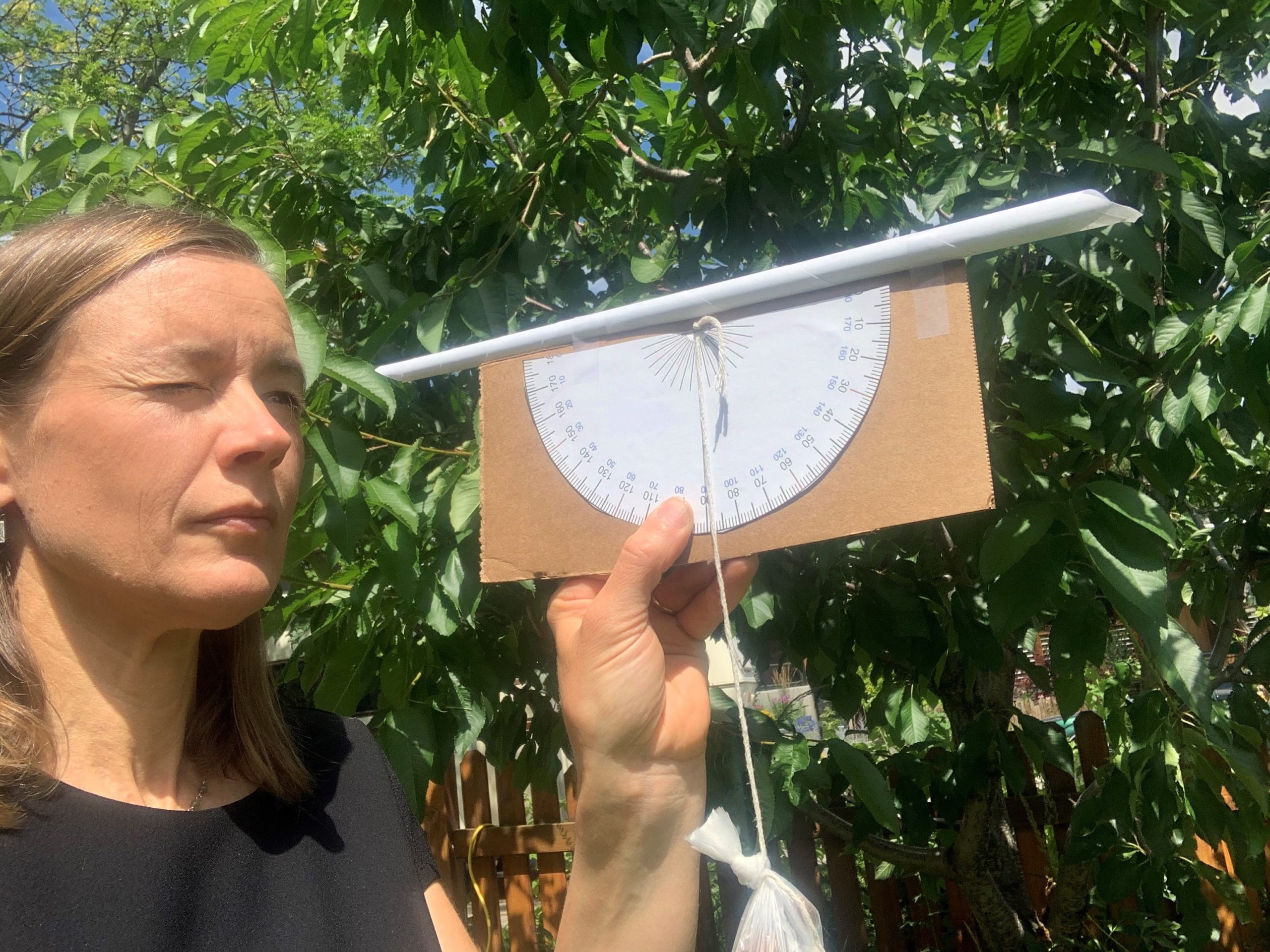
7. Level by sighting through the paper tube until the weighted string aligns with the 90⁰ line as in Figure 16.15.

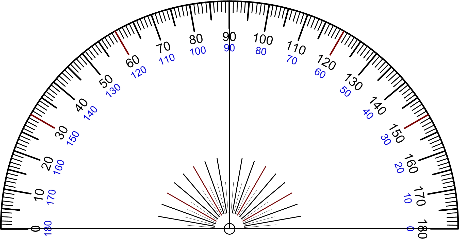
Appendix B. Protractor Template

Click the Figure 16.16 below to download.

References

Mulu, Y. & Derib, S.(2019).Positional accuracy evaluation of Google Earth in Addis Ababa, Ethiopia. Artificial Satellites, 54(2), 43-56. https://doi.org/10.2478/arsa-2019-0005

Media Attributions

• Figure 16.1: Image by C. Huscroft is licensed under a CC BY-NC-SA 4 .0 licence.
• Figure 16.2: Image by C. Huscroft is licensed under a CC BY-NC-SA 4 .0 licence.
• Figure 16.3: Image by C. Huscroft is licensed under a CC BY-NC-SA 4 .0 licence.
• Figure 16.4: Image by C. Huscroft is licensed under a CC BY-NC-SA 4 .0 licence.
• Figure 16.5: Image by C. Huscroft is licensed under a CC BY-NC-SA 4 .0 licence.
• Figure 16.6: Image by C. Huscroft is licensed under a CC BY-NC-SA 4 .0 licence.
• Figure 16.7: Image by C. Huscroft is licensed under a CC BY-NC-SA 4 .0 licence.
• Figure 16.8: Image by C. Huscroft is licensed under a CC BY-NC-SA 4 .0 licence.
• Figure 16.9: Image from Google Earth. Used in accordance with Google Earth terms and conditions.
• Figure 16.10: Image from Google My Maps (accessed June 22nd, 2020). Used in accordance with Google My Maps terms and conditions. Adapted by K. Burles.
• Figure 16.11: Image from iMapBC (accessed June 22, 2020) is © the Province of British Columbia. All rights reserved. Reproduced with permission of the Province of British Columbia. Adapted by K. Burles.
• Figure 16.12: Image from iMapBC (accessed June 22, 2020) is © the Province of British Columbia. All rights reserved. Reproduced with permission of the Province of British Columbia. Adapted by K. Burles.
• Figure 16.13: Image by K. Burles is licensed under a CC BY-NC-SA 4 .0 licence.
• Figure 16.14: Image by C. Huscroft is licensed under a CC BY-NC-SA 4 .0 licence.
• Figure 16.15: Image by C. Huscroft is licensed under a CC BY-NC-SA 4 .0 licence.
• Figure 16.16: Image by Scientif38 (2010) [JPG] is in the public domain.