Understanding Statistics
20 Inferential Statistics
Lesson
Learning Outcomes
By the end of this chapter, learners will be able to:
- define inferential statistics,
- identify examples of statistics used to measure effects of dichotomous outcomes, and
- identify examples of statistics used to measure effects of continuous outcomes.
Introduction to Inferential Statistics
Inferential statistics can help you to analyze sample data to make estimates, predictions and conclusions about populations. There are numerous statistical tests you can learn about which fall into the category of inferential statistics, but they will not all be discussed in this chapter. Instead, a sample of statistical tests you will see more commonly in research articles will be reviewed.
There are many factors to consider when determining which statistical tests should be used to analyze the results of a particular study effectively. However, we also need to ask questions to determine if the study results should be trusted to make estimates, predictions and conclusions about the population. For example, it is important to consider whether the measurements taken in the study were accurate and it is essential to determine if the sample chosen accurately represented the population. If the sample is not similar to the population, then the study results cannot be used to make predictions about what might be true for the population. You can read more about study designs, measurement and analysis in open textbooks such as Introductory Statistics, Literature Reviews for Education and Nursing Graduate Students and Scientific Inquiry in Social Work or textbooks like Nursing Research In Canada by LoBiondo-Wood, G., Cameron, C., Singh, M., & Haber, J. (2017). Assuming the study used good research methodology and is a reliable representation of the population, inferential statistics can then be used to make estimates, predictions and conclusions about what might be true for the population, based on the data from the sample.
Measuring Effect Between Outcomes
When analyzing research data, statistical tests can be used to analyze the effects of variables. For instance, they can be used to analyze the sample measurements in a study comparing the effect of two different drugs designed for potential treatment of pancreatic cancer.
The type of tests used to answer different types of questions vary. In particular, questions that have yes or no answers, or questions which have values falling on a scale, will use different types of tests. These types of answers are generally referred to as dichotomous and continuous outcomes. Dichotomous outcomes are the yes/no answer types. They relate to questions with two options for answers. For instance, does a particular medication have a potential adverse reaction of anaphylaxis? Continuous outcomes are the answer type which falls on a scale, such as how does the amount of protein in enteral feeds affect the growth of preterm infants?
Dichotomous Outcomes
There are a variety of measures that can be used to compare the effects of a variable between groups. Refer to table 20.1 to see a comparison of some of these measures.
| Statistical Test | Description |
|---|---|
| Risk | The chance of an outcome occurring. |
| Relative Risk (RR) | The comparison of the chance of an outcome occurring between two experimental groups. |
| Odds | The probability an event will occur divided by the probability of the event not occurring. |
| Odds Ratio (OR) | The probability of one event divided by the probability of another event. |
These can be tricky topics to conceptualize and challenging to determine when a particular test should be used for a specific circumstance over another. The following textboxes contain some sample scenarios to help you begin to learn about the differences in these measurements. Please note, all of the data presented in these questions are fictional and they do not represent actual measurements from real samples or studies.
Risk
Risk is a measurement of how likely an outcome will occur in a particular group, often written as a percentage. Risk is calculated by dividing the number of times the outcome occurs by the total number of cases being studied.
Risk
Let's suppose you ask, what is the chance ingesting any amount of amanita muscaria mushrooms leads to death? If you review 100 cases of known ingestion of amanita muscaria mushrooms, you might find death occurred in 5 cases.
To determine risk, the amount of times the event occurred is divided by the total amount of cases studied.
[latex]\dfrac{5}{100}= 0.05[/latex]
or 5%
Sample Exercise 20.1
Researchers are studying a new drug for potential treatment of ischemic stroke. The drug is administered to 100 mice with a known thrombus causing cerebral ischemia. Two mice suffer a fatal hemorrhage after receiving the treatment. What is the risk of fatal hemorrhage for this new fibrinolytic drug?
Answer:
[latex]\dfrac{2}{100}= 0.02[/latex]
or 2 %
Risk is calculated by dividing the number of times the event happened, by the total number of cases being studied.
Relative Risk (RR)
Relative risk is the chance of an event occurring between two groups. Relative risk is calculated by dividing the risk of the group of interest by the risk of the other group.
Values of 0 to < 1 = there is less probability of the first group having the outcome
Value of 1 = there is no difference in probability between the two groups
Values of > 1 to infinity = there is more chance of the first group having the outcome
Relative Risk (RR)
For instance, a study could review how probable antibiotic X and antibiotic Z are in curing a particular type of infection. Researchers would calculate the probability of antibiotic X in curing the infection and calculate the probability of antibiotic Z in curing the infection. Let’s say the calculated probability of antibiotic X was 98% and antibiotic Z was 85%.
[latex]\dfrac{98}{85}= 1.52[/latex]
This means antibiotic X could be 1.52 times more likely to cure the infection. However, just calculating the relative risk is not enough to say antibiotic X is the best option for treatment. We need to consider whether the study findings are statistically significant and consider many other factors about study design and potential patient outcomes before determining if antibiotic X is a good drug to use.
Choosing the Numerator and Denominator
When you set up the equation, it might be confusing to determine which risk should be the numerator and which should be the denominator. In a study where the risk for a particular group is being compared to all other groups, the particular group is the numerator and the control or comparison group is the denominator. For instance, we could compare a particular risk of an experimental treatment compared to a placebo. The risk of the experimental group would be the numerator and the risk of the group receiving the placebo would be the denominator.
Sample Exercise 20.2
A study measures the outcomes related to two drugs being used for the treatment in chronic renal failure (CRF). Drug A is an experimental drug and Drug B is one currently used in treatment of CRF. Out of 990 subjects taking drug A, 17 developed hypokalemia. Out of 998 subjects taking drug B, 32 developed hypokalemia. What is the relative risk of developing hypokalemia during treatment? What impact might this have on future use of Drugs A and B?
Answer:
Calculate the risk of hypokalemia for each drug being studied.
[latex]\dfrac{17}{990}= 0.017[/latex]
[latex]\dfrac{32}{998}= 0.032[/latex]
Calculate the relative risk by dividing the risk of hypokalemia developing with Drug A by the risk of it developing with Drug B.
[latex]\dfrac{0.017}{0.032}= 0.53[/latex]
But what does this mean? Since the value is between 0 - 1, there is less chance of hypokalemia developing with Drug A. If all other effects and characteristics of the drugs were similar, it could mean Drug A may be a better option for treatment as the risk of hypokalemia is less than Drug B.
Odds
Odds are a measure which compares the probability of something happening versus it not happening. Using odds can help people make decisions about what to do when the outcome of a particular event is uncertain. When odds are low, or close to zero, the chance of the outcome occurring are less than when the odds are high.
Odds
For instance, one might calculate the probability of nursing students graduating from a particular nursing school. In a study of 1000 BSN students, perhaps 87 students did not complete their nursing degree. That would mean that 913 students did complete their degree.
To calculate the odds, we divide the number of students who graduated by the number who did not.
[latex]\text{Odds}=\dfrac{913}{87}[/latex]
[latex]\text{Odds}=10.5[/latex]
Therefore, the odds of graduating is 10.5
Sample Exercise 20.3
What are the odds of a disease being cured if in a group of 1000 people being studied, 676 people were deemed to be cured after treatment?
Answer:
[latex]\dfrac{\text{number cured}}{\text{number not cured}}[/latex]
[latex]\dfrac{676}{324}= 2.09[/latex]
Divide the number of people cured by the number of people not cured. The odds of being cured is 2.09.
Odds Ratio (OR)
The odds ratio is used to compare the difference in odds between groups. An odds ratio of 1 would mean there is no difference between the two groups.
Odds Ratio
For instance, we could compare the odds of early births in first pregnancies in women with and without gestational diabetes (GD). Let’s suppose that 16/100 women with GD delivered prematurely and 5/100 women without GD delivered early.
We first need to calculate the odds of each group:
Odds premature delivery of first pregnancy in women with GD = 0.19
Odds premature delivery of first pregnancy without GD =0.052
[latex]\text{Odds Ratio}=\dfrac{0.19}{0.052}[/latex]
[latex]\text{Odds Ratio}= 3.65[/latex]
This number indicates it is 3.65 times more likely for a premature birth to occur early in a first pregnancy for someone with gestational diabetes.
Sample Exercise 20.4
Researchers compare the effects of taking two nutritional supplements while studying the rate of healing of pressure ulcers. They find supplement A improves average healing time by at least 7 days in 32/100 cases and supplement B improves average healing time by at least 7 days in 4/100 cases.
Answer:
Calculate the probability of average healing time improving by at least 7 days for each nutritional supplement.
[latex]\dfrac{32}{100}= 0.32[/latex] or 32 %
[latex]\dfrac{4}{100}= 0.04[/latex] or 4 %
Divide the probability of improvement with supplement A by the probability of improvement with supplement B.
[latex]\dfrac{32}{4}= 8[/latex]
The odds ratio of 8 shows a value > 1, meaning there is more chance of improvement with supplement A.
Continuous Outcomes
Two common types of statistics which help us determine the validity of study findings are p-values and confidence intervals. P-values can help us to determine how often the effect found in a study is more or less likely to be due to random chance than being a true finding and confidence intervals can tell us about the replicability of results.
P-Values
Researchers look for associations between variables and effects in studies and will calculate statistics, like p-values, to help determine if an effect found is actually a true finding. Calculation of p-values help determine if study results are just a coincidence by estimating what chance there is of the effect found to be related to sampling error during the study process.
P-values exist on a scale. The higher the p-value, the less certain one can be regarding the true effect of the variable. The lower the p-value, the more likely the results are representative of an actual effect and less likely results are just a coincidental finding. It is important to note one study with a low p-value does not prove conclusively that the results are true for the population. The more studies which show a low p-value, the more likely the results can be applied to conclusions about the population.
P-values belong in a category of statistical tests called hypothesis tests. This category of tests helps researchers to determine if they accept or reject a hypothesis. When setting up a study, the researcher will write a null hypothesis (H0) and an alternate hypothesis (HA). The null hypothesis describes a circumstance in which the variable does not have an effect on the outcome being studied. The alternate hypothesis describes a circumstance in which the variable has an effect.
Sample Hypothesis Statements
H0: Drinking caffeine increases in systolic blood pressure by less than 5 mmHg.
HA: Drinking caffeine increases blood pressure by at least 5 mmHg.
These statements can be abbreviated like this:
H0: < 5
HA: ≥ to 5
The p-value statistic always assume the null hypothesis is true. If p-values are higher, the study results are consistent with a true null hypothesis, meaning the study did not find any evidence of the variable having an actual effect. In this case, the researcher would state they accept the null hypothesis. If the p-values are small, the study results are not consistent with the null hypothesis. If this is the case, it means the thing being studied either has an effect or there may have been sampling error influencing the study results and the effect found is actually just a coincidence. The researcher would state the null hypothesis is rejected.
In order to make a decision to accept or reject the null hypothesis, the researchers must determine the level of certainty they will accept in order to consider the findings statistically significant and apply the study findings to inferences about the population. They determine this level, and call it the alpha (α) value. An alpha value can be anywhere between 0 - 1, with lower numbers having a higher degree of certainty. In many studies, the alpha value is often 0.05. Other studies might set the alpha value to 0.01. If the calculated p-value is less than alpha, then the null hypothesis is rejected. Recall that the lower the p-value, the more certain one can be an effect is a true finding and not a finding produced by a random sampling error. It is still possible a p-value lower than alpha could indicate the results were produced due to a sampling error, hence why the researcher say the reject the null hypothesis versus they accept the alternate hypothesis. Consequently, the more studies able to replicate the results, the more certain we are about the validity of the findings.
Accepting or Rejecting a Null Hypothesis
A study is undertaken to measure the effect of a new treatment for muscle rigidity in Parkinson's disease. Measurements of muscle rigidity are taken with clinical instruments to obtain an objective measurement. Alpha is set to 0.01. The calculated p-value is 0.0082.
H0: there is no difference in muscle rigidity measurements at rest
HA: there is at least a 5% decrease in muscle rigidity measurements at rest
Based on the calculated p-value, does the researcher accept or reject the null hypothesis?
Since the p-value is lower than alpha, the researcher rejects the null hypothesis.
P-values are measured with different types of statistical tests depending on the number and type of variables being studied. Table 20.2 depicts the types of statistical tests to calculate p-values for various types of data. Future courses in statistics will help you learn how to calculate these measures to aid in analyzing study results.
| Type of Data | Statistical Test |
|---|---|
| 1 Category | 1 Sample Proportion Test |
| 2 Categories | Chi Squared Test |
| 1 Numeric | T-test |
| 1 Numeric and 1 Category | T-test, 1 way ANOVA |
| 1 Numeric and 2 Categories | 2 way ANOVA |
| 2 Numeric | Correlation Test |
Sample Exercise 20.5
A study is undertaken to measure the effect of a potential new drug for hypercholesterolemia.. Alpha is set to 0.01. The calculated p-value is 0.18.
H0: there is no change in serum LDL levels
HA: there is a decrease in serum LDL levels by ≥ 20 mg/dL
Based on the calculated p-value, does the researcher accept or reject the null hypothesis?
Answer:
Since the p-value is higher than alpha, the researcher accepts the null hypothesis.
Confidence Intervals
Confidence intervals help to give an idea of how well the sample statistic represents a population parameter. They describe the range in which the true population parameter is likely to be in and give the probability of how often it would be found in the range. Examples of sample statistics with confidence intervals could be data like the mean, odds ratio, or relative risk.
In a study, is it highly unlikely the reported sample statistic will match the true population parameter because not all of the measurements from the population are included in the calculation. Inherently, there is some degree of measurement error which will occur from using a sample. The more the characteristics of the sample correlate with the characteristics of the population, the smaller the amount of error. Taking larger samples may also reduce error and lead to more precise estimates of the actual population parameter. Confidence intervals can have a very small or very large range of minimum and maximum interval values, depending on how precise the estimate is. The more precise the estimate, the smaller the range of the confidence interval will be.
The two numbers in the interval represent values which are a certain number of standard deviations above and below the sample statistic. The number of standard deviations chosen is related to the percentage of confidence noted. Recall, in a normal distribution, 95% of the values will be within two standard deviations of the point estimate. If three standard deviations above and below are considered, this equates to 99.7% of the values. Most often, you will see confidence intervals which note the 95% level of confidence.
Interpreting Confidence Intervals
In a study measuring the average time for epinephrine to reduce hives associated with anaphylaxis, a statement in the research article might say:
“There is a 95% confidence interval that IV administration of epinephrine will reduce hives within five to seven minutes of administration.”
It may be abbreviated like this: 95% CI 6 (5, 7)
This means if the same experiment was repeated many times, 95% of the time the population mean will fall within the range of five to seven minutes.
Sample Exercise 20.6
A study is completed measuring the prevalence of pre-test exam related anxiety at a particular university. Prevalence is reported as a percentage of students. Study data is analyzed and a researcher reports the following:
95% CI 29.6% (24.4, 34.8)
Explain the above statistic in your own words. What do each of the numbers represent?
Answer:
Based on the data collected from study participants, 29.6% of students reported pre-test exam related anxiety. 29.6% is not likely to be the exact percentage of the true prevalence of anxiety in all students at the university due to error from using a sample of the population. The researcher is giving a range of values in which they are 95% certain the actual population prevalence of pre-test anxiety falls within. The range is 24.4-34.8 %.
Meta-analysis
In recent years, more health care providers are seeking to use the results of multiple studies investigating the effect of a particular variable on a specific outcome when making decisions regarding best practice. Egger and Smith (1997) describe metanalysis as “the statistical integration of separate studies.” A basic process for metanalysis would include the following steps:
- The researcher considers what research question they are trying to answer. They must be able to articulate the specific qualities of the intervention and the characteristics of the population being studied. Defining the variables and outcomes being studied explicitly help the researcher in the next step of the process.
- A thorough literature review is conducted to find reports of studies which help to answer the research question. Studies which look at a particular intervention but are studying different populations cannot be analyzed together. Think about this step as ensuring you are comparing apples to apples. Some studies may not be comparable to each other and therefore would not be included in the actual metanalysis. It can be very challenging to find studies which have populations with characteristics similar enough to be able to be analyzed together, so there may be times when a literature review does not proceed to the next steps of meta-analysis.
- The researcher uses statistical analysis to compare the results of studies deemed to be homogeneous.
- A report is written to present the summary of findings and methods of statistical analysis.
Forest Plots
Forest plots are used to graphically summarize the comparison of results of multiple studies used in a meta-analysis. The forest plot has data relating to each individual study included in the analysis and a representation of the combined study results. It helps to predict if the combined results of studies lean towards the subject having a true effect or not.
There are several standard features of forest plots:
Square: A square shape is used to depict the results from one study. The size of the square is related to the sample size of the study. Squares of each study on the forest plot will differ in size, depending on the sample size used in each study. For instance, bigger squares quickly indicate that the sample sizes of those studies were larger.
Diamond: A diamond shape is used to indicate the combined estimated effect of the study results. On a graph, the center of the diamond equates to the value of the calculated statistic. The point at the furthest left and furthest right equate to the values of the confidence interval for the calculated statistic. The longer the width of the diamond, the more range there is in potential true value. Therefore, a diamond with a shorter width has a potential true value in a smaller range.
Line of No effect: On the forest plot there will be a vertical line depicting the value at which the variables have no effect on the outcome. The value depends on the statistic that is being compared. For instance, if odds ratio is being measured, there is no difference in effect when the odds ratio equals one, so the line of no effect is placed at one on the x axis. Study results which have a confidence interval crossing the line of no effect are considered to not be statistically significant, as there is a chance the variable has no effect on the outcome.
Horizontal lines: Indicate the confidence interval calculated for each study.
See image below to review some standard features of a forest plot:
Sample Exercise 20.7
Refer to the image of the sample forest plot to answer the following questions:
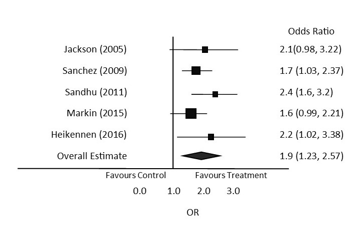
- Which individual study has the smallest sample size?
- What is the calculated odds ratio of the overall estimate?
- Which individual studies are statistically significant?
- If the odds ratio of > 1 favours the treatment over the control, does this summary of study data suggest the treatment has an effect on the outcome being studied?
Answers:
- Sandhu (2011). The sample size correlates to the size of the square. It is the smallest square on the forest plot, therefore it has the smallest sample size.
- 1.9
- The studies by Sanchez, Sandhu and Heikennen. They are considered statistically significant because the confidence interval does not cross the line of no effect.
- Yes. The diamond is to the right of the line of no effect, and the graph is labelled as favouring treatment on the right side of the line of effect.
Critical Thinking Questions
- If a finding is considered statistically significant, should we then conclude this is something which should now be adopted as part of our practice?
- In a particular study, if alpha = 0.01, are the researchers seeking more or less certainty in their findings than if alpha = 0.05?
Answers:
- Not necessarily, there are more factors to consider that just statistical significance of an effect. Additional analysis should be undertaken to determine if a particular approach should be used, and the type of analysis will depend on the subject of the study. For instance, if you were considering whether or not to use a new drug, you would also need to analyze for potential serious adverse reactions and determine if it is a cost-effective treatment.
- The researchers are looking for more certainty when determining whether or not to reject the null hypothesis. If p = 0.01, this would mean there is a 1% chance of the null hypothesis being true.
Key Takeaways
- Inferential statistics is used to analyze sample data when making estimates, predictions and conclusions about populations.
- Risk is a measurement of how likely an outcome will occur in a particular group, often written as a percentage.
- Relative risk is the chance of an event occurring between two experimental groups.
- Odds are a measure which compares the probability of something happening versus it not happening.
- The odds ratio is used to compare the difference in odds between groups.
- P-values are calculated to help identify if a null hypothesis should be accepted or rejected. They help determine if study results are just a coincidence by estimating what chance there is of the effect found to be related to sampling error.
- Confidence intervals of a sample statistic describe the range in which the true population parameter is likely to be in and give the probability of how often it would be found in the range.
- Meta-analysis is a process used to for statistical analysis of data pooled from comparable studies.
- Forest plots are used to graphically summarize the comparison of results of multiple studies used in a meta-analysis.
Practice Set 20.1: Calculating Risk
Practice Set 20.1: Calculating Risk
Calculate the risk in the following scenarios.
- 1,000 people are exposed to a particular protozoa while swimming in a tropical lake. 54 people become infected and exhibit symptoms of disease. What is the risk of developing the disease?
- A study is completed to review the risk of a particular disease developing during childhood. 100,000 cases were reviewed and it was found that 3,411 children developed the disease. What is the risk of developing the disease?
- 150,000 people in a small town use a particular reservoir for all of their drinking water. A toxic spill occurs in the reservoir and 2, 347 people suffer with symptoms of poisoning. What is the risk of being poisoned by this substance?
- Researchers review 10,000 cases of people who were diagnosed with a particular cancer. 8,984 people survived 5 years after treatment was complete. What is the risk of death within 5 years of completion of treatment?
- A new drug is being tested for treatment of hypertension. Researchers determine the drug is effective at reducing blood pressure, but are concerned with the possibility of severe adverse reactions. Of the 100 people who receive the drug, researchers determine 7 people have severe adverse reactions. What is the risk of developing a severe adverse reaction?
Answers:
- [latex]\dfrac{54}{1000}= 0.05[/latex] or 5%
- [latex]\dfrac{3411}{100000}= 0.03[/latex] or 3%
- [latex]\dfrac{2347}{150000}= 0.02[/latex] or 2%
- [latex]\dfrac{1016}{10000}= 0.1[/latex] or 10%
- [latex]\dfrac{7}{100}= 0.07[/latex] or 7%
Practice Set 20.2: Calculating Relative Risk
Practice Set 20.2: Calculating Relative Risk
Calculate relative risk for the following questions and write a statement in your own words describing the relative risk.
- Two treatments for stage 3 ovarian cancer are being compared. A new treatment, treatment A, has a probability of 10 year survival of 88 %. The current treatment, treatment B, is 67 %.
- Cure of a fungal nail infection is determined to be 0.62 with drug A and 0.45 with drug B.
- Two drugs for the treatment of pulmonary embolism are being studied. The probability of resolution of the embolism is 0.7 for drug A and 0.87 for drug B.
- The risk of nephropathy after using a particular contrast dye, "dye x" for CT preparation in people with diabetes is 32 %. The calculated risk of the control group is 21%.
- The risk of a serious birth defect occurring for treatment of a maternal infection during the first trimester with drug X is 0.003 and is 0.011 for drug Y.
Answers:
- [latex]\dfrac{88}{67}= 1.31[/latex]
The 10 year survival rate using treatment A compared to treatment B is increased by 1.3 fold. - [latex]\dfrac{0.62}{0.45}= 1.38[/latex]
drug A is 1.38 times more likely to cure the fungal nail infection than drug B. - [latex]\dfrac{0.7}{0.87}= 0.82[/latex]
The likelihood of resolution of a pulmonary embolism using drug A is 0.8 times less likely than using drug B. - [latex]\dfrac{32}{21 }= 1.52[/latex]
The risk of nephropathy after using contrast dye "X" in people with diabetes is 1.52 times more likely than those without diabetes. - [latex]\dfrac{0.003}{0.011}= 0.27[/latex]
The risk of developing a serious birth defect during the first trimester, while treating a maternal infection, is 0.27 times less likely with drug X.
Practice Set 20.3: Calculating Odds
Practice Set 20.3: Calculating Odds
Calculate the odds in the following scenarios.
- Self reported patient anxiety is reduced by at least 3 points on a scale of 1 - 10 after the nurse guides the patient through a deep breathing exercise in 945 out of 1000 cases.
- Heart disease develops after daily use of a new sugar substitute over a one year period in 7/100 cases studied.
- In a study measuring the occurrence of febrile seizures in children 5 years and younger, researchers determined out of 1000 children with a particular illness resulting in fever, 49 experienced a febrile seizure.
- A year long research study was being conducted on a potential new treatment for myalgic encephalomyelitis. The treatment resulted in improvement of daily fatigue ratings during the study period in 211 out of 500 cases.
- A study of a new dietary treatment plan for drug-resistant epilepsy found 77 of 1000 people attained six months being seizure free.
Answers:
- [latex]\dfrac{945}{55}= 17.2[/latex]
- [latex]\dfrac{7}{93}= 0.08[/latex]
- [latex]\dfrac{49}{951}= 0.05[/latex]
- [latex]\dfrac{211}{289}= 0.73[/latex]
- [latex]\dfrac{77}{923}= 0.08[/latex]
Practice Set 20.4: Calculating Odds Ratio
Practice Set 20.4: Calculating Odds Ratio
Calculate the odds ratio for the following scenarios.
- Self reported patient anxiety is reduced by at least 3 points on a scale of 1 - 10 after the nurse guides the patient through a deep breathing exercise in 945 out of 1000 cases. An alternate deep breathing exercise reduced anxiety by at least 3 points on a scale of 1 - 10 in 722 out of 987 cases.
- Heart disease develops after daily use of a new sugar substitute over a one year period in 7/100 cases studied. A commonly used sugar substitute was also studied, and researchers found heart disease developed in 1/100 cases.
- Researchers measure the effect of two potential new drugs for the treatment of neuropathic pain. Drug A achieved a reduction of moderate pain to mild pain in 32/100 cases. Drub B achieved a reduction of moderate pain to mild pain in 15/100 cases.
- The effects of two exercise programs on increasing range of motion (ROM) during the rehabilitation phase of a grade 3 ankle sprain are studied. Researchers find that participants using exercise program A achieved an acceptable ROM in 82/98 cases. Participants using exercise program B achieved an acceptable ROM in 84/100 cases.
- A study is measuring the severity of nausea in two chemotherapy drugs with similar effectiveness in treating a particular cancer. Researchers find study participants receiving chemotherapy drug A have a nausea rating of at least 4 on a scale of 0-10 in 645/978 cases. Participants receiving chemotherapy drug B have a nausea rating of at least 4 in 552/967 cases.
Answers:
- Calculate the odds for each study group. Divide the odds of the first group by the odds of the second group. The odds ratio is 6.4
[latex]\dfrac{945}{55}= 17.2[/latex][latex]\dfrac{722}{265}= 2.7[/latex][latex]\dfrac{17.2}{2.7}= 6.4[/latex] - The odds ratio is 8
[latex]\dfrac{7}{93}= 0.08[/latex][latex]\dfrac{1}{99}= 0.01[/latex][latex]\dfrac{0.08}{0.01}= 8[/latex] - The odds ratio is 2.6
[latex]\dfrac{32}{68}= 0.47[/latex][latex]\dfrac{15}{85}= 0.18[/latex][latex]\dfrac{0.47}{0.18}= 2.6[/latex] - The odds ratio is 0.98
[latex]\dfrac{82}{16}= 5.13[/latex][latex]\dfrac{84}{16}= 5.25[/latex][latex]\dfrac{5.13}{5.25}= 0.98[/latex] - The odds ratio is 1.46
[latex]\dfrac{645}{333}= 1.94[/latex][latex]\dfrac{552}{415}= 1.33[/latex][latex]\dfrac{1.94}{1.33}= 1.46[/latex]
Practice Set 20.5: P-Values Fill in the Blanks
Practice Set 20.5: P-Values Fill in the Blanks
Practice Set 20.6: Interpreting P-Values
Practice Set 20.6: Interpreting P-Values
For the following questions, state if the p-value is considered to be statistically significant. Is the null hypothesis accepted or rejected?
- A study is undertaken to compare the effect of a particular variable on the development of atrial fibrillation compared to a control group. Alpha is 0.01. The P-value is 0.27.
- A researcher presents the results of a study. Alpha is 0.01. The P-value is 0.012.
- A study is undertaken to compare the effect of a particular variable on the development of ulcerative colitis compared to a control group. Alpha is 0.01. The P-value is 0.003.
- A researcher presents the results of a study. Alpha is 0.05. The P-value is 0.077.
- A study is undertaken to compare the effect of a particular variable on the development of multiple sclerosis compared to a control group. Alpha is 0.05. The P-value is 0.038.
- A researcher presents the results of a study. Alpha is 0.01. The P-value is 0.0026.
- A study is undertaken to compare the effect of a particular variable on the development of Parkinson's disease compared to a control group. Alpha is 0.01. The P-value is 0.87.
- A researcher presents the results of a study. Alpha is 0.01. The P-value is 0.25.
- A study is undertaken to compare the effect of a particular variable on the incidence of asthma compared to a control group. Alpha is 0.05. The P-value is 0.016.
- A researcher presents the results of a study. Alpha is 0.05. The P-value is 0.096.
Answers:
- The P-value is not statistically significant and the null hypotheses is accepted.
- The P-value is not statistically significant and the null hypotheses is accepted.
- The P-value is statistically significant and the null hypotheses is rejected.
- The P-value is not statistically significant and the null hypotheses is accepted.
- The P-value is statistically significant and the null hypotheses is rejected.
- The P-value is statistically significant and the null hypotheses is rejected.
- The P-value is not statistically significant and the null hypotheses is accepted.
- The P-value is not statistically significant and the null hypotheses is accepted.
- The P-value is statistically significant and the null hypotheses is rejected.
- The P-value is not statistically significant and the null hypotheses is accepted.
Practice Set 20.7: Confidence Intervals
Practice Set 20.7: Confidence Intervals
- If the sample size of a study was increased, what is likely to happen to the size of the confidence interval? Why?
- Data is collected to estimate how many hours of sleep fourth year nursing students receive per night. Researchers report a 95% CI of a population mean between 6.8 - 8.7. Is it possible that the average amount of sleep per night is less than 6.8?
- For a confidence interval reporting 99.7% confidence, how many standard deviations away from a sample mean are used to determine the interval numbers?
- Study data is analyzed comparing a placebo to a treatment for the reduction of pregnancy related nausea, with numbers lower than 1 favouring the placebo. The following statistics are reported:
Odds ratio 1.57 (1.27, 1.87) with 95% CI
Explain the above statistic in your own words. What do each of the numbers represent?
- A study is completed to explore the effects of a variety of birth control methods on menstrual pain. One effect researchers were curious about was the highest level of pain reported in each menstrual cycle over a period of one year. Pain is measured on a scale of 0-10 and the following results are reported:
Control Group 95% CI 3.8 (3.1, 4.5)
Option A 95% CI 5.6 (5.2, 6.0)
Option B 95% CI 3.9 (2.9, 4.9)
Option C 95% CI 2.1 (1.5, 3.6)
a. What is the average highest pain rating for the control group?
b. Is there a group whereby the sample mean indicates a lower rating of pain than the control? If so, which group?
c. Is there a group whereby the population mean is likely to be higher than the control group? If so, which group?
d. If the researchers wanted to report a 99.7% confidence interval, what would happen to the size of the intervals for each group?
Answers:
- The confidence interval would likely decrease because as the sample size is increased, the amount of standard error is reduced. (Assuming the sample taken remains a random sample of the population).
- Yes, it is possible the true population mean is outside of the reported range. It can be higher or lower than the reported interval, therefore it could be less than 6.8.
- To report with 99.7% confidence, a statistician would use the numbers three standard deviations above and below the sample mean to determine the confidence interval.
- The treatment is estimated to be 1.57 times more likely to reduce nausea than the placebo. In 95% of well chosen samples, the true odds ratio will fall in the range of 1.27 to 1.87.
- a. 3.8/10
b. Option C
c. Option A
d. The size of the intervals would increase, as the intervals reported would need to be 3, instead of 2, standard deviations away from the sample mean.
Practice Set 20.8-20.9: Interpreting Forest Plots
Practice Set 20.8: Interpreting Forest Plots
The image below depicts a forest plot comparing the results of multiple studies. Refer to the image of the sample forest plot to answer the following questions:
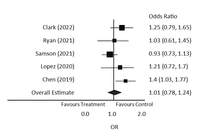
- What does the vertical line represent?
- Are the findings of this meta-analysis considered to be statistically significant?
- Which study has the largest effect on the overall summary?
- Which study or studies have significant results?
Answers:
- The line of no effect.
- No, the diamond shape crosses the vertical line of no effect, so the results are not considered to be statistically significant.
- Samson (2021)
- Chen (2019) is the only study with statistically significant results because it does not cross the line of no effect.
Practice Set 20.9: Interpreting Forest Plots
The image below depicts a forest plot comparing the results of multiple studies. Refer to the image of the sample forest plot to answer the following questions:
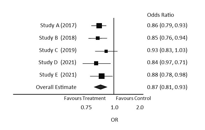
- What study has the smallest sample size?
- Is the overall summary considered to be statistically significant?
- Which individual studies are considered to be statistically significant?
- Which study has the largest confidence interval?
Answers:
- Study C
- Yes, it does not cross the line of no effect.
- Study A, B, D and E are statistically significant as they do not cross the line of no effect.
- Study D
Outcomes which have only two possible options.
Outcomes which have numerous possible outcomes, measured on a scale.
The chance of an outcome occurring.
The comparison of the chance of an outcome occurring between two experimental groups.
The probability an event will occur divided by the probability of the event not occurring.
The probability of one event divided by the probability of another event.
A calculated statistic to help determine if study results are just a coincidence by estimating what chance there is of the effect found to be related to sampling error during the study process.
A statistic which describes the range in which the true population parameter is likely to be in and gives the probability of how often it would be found in the range.
A statement describing a circumstance where there is no difference between the variables being studied.
A statement about a population that is contradictory to the null hypothesis, in which a variable has an effect on an outcome being studied.
A graph summarizing the comparison of results of multiple studies used in a meta-analysis. The forest plot has data relating to each individual study included in the analysis and a representation of the combined study results.
