Chapter 5: Systems of Equations
5.1 Graphed Solutions
Often, it is necessary to find the coordinates that are shared by two or more equations. There are multiple methods to find these shared values. While not giving values that are precise, graphing these equations make it possible to see the approximate solution and what type of solution it is.
Problems like [latex]3x - 4 = 11[/latex] have been solved in this textbook by adding 4 to both sides and then dividing by 3 (solution is [latex]x = 5[/latex]). There are also methods to solve equations with more than one variable in them. It turns out that, to solve for more than one variable, it is necessary to have the same number of equations as variables. For example, to solve for two variables such as [latex]x[/latex] and [latex]y,[/latex] two equations are required. When there are several equations that must be solved, that is called a system of equations. When solving a system of equations, the solution must work in both equations. This solution is usually given as an ordered pair, [latex](x, y).[/latex] The following example illustrates a solution working in both equations.
Example 5.1.1
Show [latex](2, 1)[/latex] is a solution to the equations [latex]3x - y = 5[/latex] and [latex]x + y = 3.[/latex]
Using the coordinates [latex](2, 1),[/latex] check to see if [latex]x = 2,[/latex] [latex]y = 1[/latex] is a solution for both equations.
[latex]\begin{array}{rr} \begin{array}{rr} \\ \text{For }3x-y=5\hspace{0.2in}&3(2)-(1)=5 \\ &6-1=5 \\ &5=5 \end{array} &\hspace{0.25in} \begin{array}{rr} \text{For }x+y=3\hspace{0.2in}&(2)+(1)=3 \\ & 3=3 \end{array} \end{array}[/latex]
The coordinate [latex](2, 1)[/latex] is a solution for both equations, which means that the lines that they represent will intersect at [latex](2, 1)[/latex] when they are drawn on a graph.
Note that the graph of an equation yields a picture of all its solutions. When two equations are graphed on the same coordinate plane, this displays not only the solutions of both equations, but where these solutions intersect. For instance, these solutions will show if the linear equations intersect at a point, over a line, or not at all.
In the following examples, each of the three possible types of solutions will be explored.
Example 5.1.2
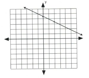
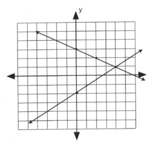
Identify if any common intersection exists between the following linear equations: [latex]y = -\dfrac{1}{2}x + 3[/latex] and [latex]y = \dfrac{3}{4}x - 2.[/latex]
First, graph [latex]y = -\dfrac{1}{2}x + 3.[/latex] The slope is [latex]-\dfrac{1}{2}[/latex] and the [latex]y[/latex]-intercept is 3. For the first point, choose the intercept, and choose the second one using the slope. Draw a line through these two points to generate the first line.

Now, graph the second equation, [latex]y = \dfrac{3}{4}x - 2[/latex], using its slope of [latex]\dfrac{3}{4}[/latex] and intercept of −2.

The lines cross at the coordinate [latex](4, 1).[/latex]
To check to see if this intersection is correct, substitute [latex]x = 4[/latex] and [latex]y = 1[/latex] into the two original equations.
[latex]\begin{array}{rr} \begin{array}{rrrl} \text{Check:}\hspace{0.5in}&y&=&-\dfrac{1}{2}x+3 \\ \\ &(1)&=&-\dfrac{1}{2}(4)+3 \\ \\ &1&=&-2+3 \\ \\ &1&=&1 \end{array} &\hspace{0.25in} \begin{array}{rrl} y&=&\dfrac{3}{4}x-2 \\ \\ (1)&=&\dfrac{3}{4}(4)-2 \\ \\ 1&=&3-2 \\ \\ 1&=&1 \end{array} \end{array}[/latex]
The coordinate [latex](4, 1)[/latex] is the shared point between both linear equations. This type of intersection is a unique solution that is called consistent and independent.
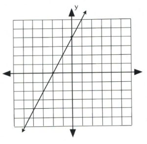
It is also possible to have a situation in which the same linear equation is graphed twice. Such an equation is easy to create.
Take the equation [latex]y = 2x + 1[/latex]:
[latex]\begin{array}{l} \text{Multiplying by 2 results in } 2y = 4x + 2 \\ \text{Multiplying by 3 results in } 3y = 6x + 3 \\ \text{Multiplying by }\dfrac{1}{2}\text{ results in }\dfrac{1}{2}y = x + \dfrac{1}{2}\\ \text{Multiplying by } -2 \text{ results in } -2y = -4x - 2 \end{array}[/latex]
These are all the same equation, and if any two of them were graphed, the result would be the exact same line. This type of intersection has many solutions and is called consistent and dependent.
Example 5.1.3
Find the intersection of the linear equations [latex]2x - y = -4[/latex] and [latex]4x - 2y = -8.[/latex]
Plot these equations using their intercepts:

For [latex]2x - y = -4[/latex]:
when [latex]x = 0, y = 4\hspace{0.35in} (0, 4)[/latex]
when [latex]y = 0, x = -2\hspace{0.25in} (-2, 0)[/latex]
For [latex]4x - 2y = -8[/latex]:
when [latex]x = 0, y = 4\hspace{0.35in} (0, 4)[/latex]
when [latex]y = 0, x = -2\hspace{0.25in} (-2, 0)[/latex]
The two lines from the previous example have the exact same intercepts and, when graphed, draw the exact same line. Since the two graphs have solutions, it is defined as being consistent. However, the many solutions means they are dependent.
Lines that are parallel will never intersect and, as a result, will never have a solution or a shared intersection. Any system of equations having no solution is defined as being inconsistent. Parallel equations are identical except for having different intercepts. This means that the equation [latex]2x + 3y = 5[/latex] is parallel to:
[latex]2x + 3y = 6\hspace{0.25in} 2x + 3y = 7\hspace{0.25in} 2x + 3y = 8\hspace{0.25in} 2x + 3y = 0\hspace{0.25in} 2x + 3y = -5[/latex]
Each of the above equations is parallel and will never intersect with each other.
Example 5.1.4
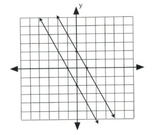
Find the intersection of the linear equations [latex]2x + y = -2[/latex] and [latex]2x + y = 2.[/latex]
Plot these equations using their intercepts:

For [latex]2x + y = -2[/latex]:
when [latex]x = 0, y = -2\hspace{0.25in} (0, -2)[/latex]
when [latex]y = 0, x = -1\hspace{0.25in} (-1, 0)[/latex]
For [latex]2x + y = 2[/latex]:
when [latex]x = 0, y = 2\hspace{0.25in} (0, 2)[/latex]
when [latex]y = 0, x = 1\hspace{0.25in} (1, 0)[/latex]
Questions
For questions 1 to 12, find the intersection point of each system of equations.
- [latex]\left\{ \begin{array}{rrrrr} y&=&-x&+&1 \\ y&=&-5x&-&3 \end{array}\right.[/latex]
- [latex]\left\{ \begin{array}{rrrrr} y&=&-\dfrac{5}{4}x&-&2 \\ \\ y&=&-\dfrac{1}{4}x&+&2 \end{array}\right.[/latex]
- [latex]\left\{ \begin{array}{rrrrr} y&=&-3&& \\ y&=&-x&-&4 \end{array}\right.[/latex]
- [latex]\left\{ \begin{array}{rrrrr} y&=&-x&-&2 \\ y&=&\dfrac{2}{3}x&+&3 \end{array}\right.[/latex]
- [latex]\left\{ \begin{array}{rrrrr} y&=&-\dfrac{3}{4}x&+&1 \\ \\ y&=&-\dfrac{3}{4}x&+&2 \end{array}\right.[/latex]
- [latex]\left\{ \begin{array}{rrrrr} y&=&2x&+&2 \\ y&=&-x&-&4 \end{array}\right.[/latex]
- [latex]\left\{ \begin{array}{rrrrr} y&=&\dfrac{1}{3}x&+&2 \\ \\ y&=&-\dfrac{5}{3}x&-&4 \end{array}\right.[/latex]
- [latex]\left\{ \begin{array}{rrrrr} y&=&2x&-&4 \\ y&=&-4x&+&2 \end{array}\right.[/latex]
- [latex]\left\{ \begin{array}{rrrrr} y&=&\dfrac{5}{3}x&+&4 \\ \\ y&=&-\dfrac{2}{3}x&-&3 \end{array}\right.[/latex]
- [latex]\left\{ \begin{array}{rrrrr} y&=&-\dfrac{1}{2}x&+&4 \\ \\ y&=&-\dfrac{1}{2}x&+&1 \end{array}\right.[/latex]
- [latex]\left\{ \begin{array}{rrrrr} x&+&3y&=&-9 \\ 5x&+&3y&=&3 \end{array}\right.[/latex]
- [latex]\left\{ \begin{array}{rrrrr} x&+&4y&=&-12 \\ 2x&+&y&=&4 \end{array}\right.[/latex]

