Learning Task 2
Select and Size Piping
Tubing Layout Patterns
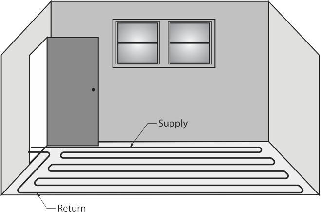
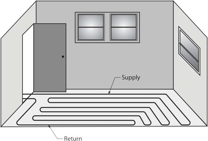
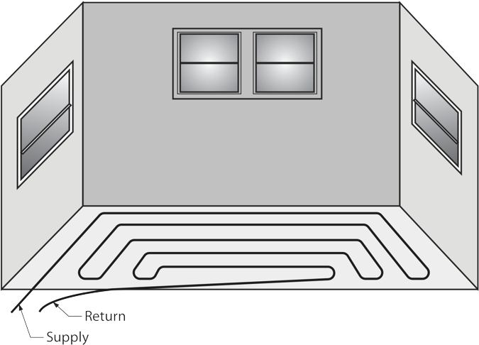
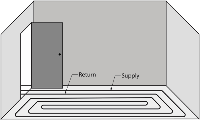
The graphics above show the common floor panel tubing layouts used. The layout chosen will primarily depend upon the room itself, which could have up to six unheated environments butting up to it. For instance, if a room has an unheated carport below or an unheated attic space above, a counterflow pattern is a good choice in that it spreads the heat out evenly across the floor. Serpentine layouts are common for rooms with 1 or 2 outside walls.
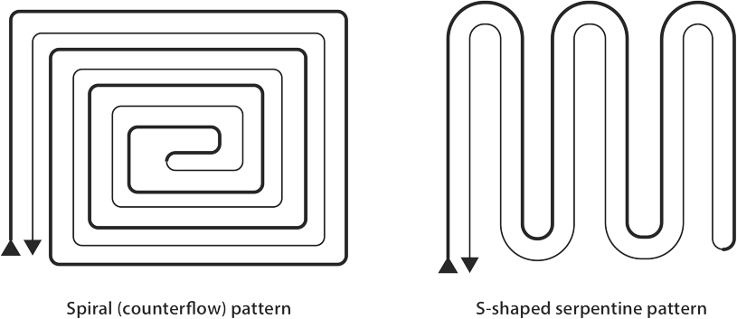
The main consideration in the loop layouts is that the warmest water should always be delivered to the areas of greatest heat loss first, so the tubing should enter a room through the doorway and make one pass along the outside wall or walls, about 6 inches from them. Then, the tubing turns 180° and parallels the first run at a distance of 6 inches away from the first pass. After the initial 2 passes, the installer then resumes with the layout pattern chosen.
Tube Size and Loop Spacing
A loop is a run of tubing that starts at the supply manifold and ends at the return manifold. Loop centre spacing is determined by the size of the tube and the required floor output in BTUH/ft² of available area. Excluding the spacings at outside walls, spacing for residential systems can vary between 12″, 9″, 6″ and in a few cases even as narrow as 4″ on centre. Commercial systems can be greater than 12″ o.c. where tubing of [latex]\dfrac{5}{8}[/latex]″ NPS and larger is used. Although tubing of [latex]\dfrac{1}{4}[/latex]″ NPS and [latex]\dfrac{3}{8}[/latex]″ NPS has special applications, tubing of [latex]\dfrac{1}{2}[/latex]″ NPS is the standard size for residential systems. Table 2.1 below shows the relationship between tube diameter and spacing.
| Floor Output Required | Tube Diameter (Nominal I.D.) | |||
|---|---|---|---|---|
| BTUH/sq ft | [latex]\dfrac{3}{8}[/latex]″ | [latex]\dfrac{1}{2}[/latex]″ | [latex]\dfrac{5}{8}[/latex]″ | [latex]\dfrac{3}{4}[/latex]″ |
| 0 – 10 | 12 | 12 | 12 | 12 |
| 10 – 20 | 9 | 12 | 12 | 12 |
| 20 – 25 | 9 | 12 | 12 | 12 |
| 25 – 30 | 6 | 9 | 12 | 12 |
| 30 – 40 | 4 | 6 | 9 | 9 |
As you can see, residential ½″ tubing is installed at 12″ on centre for heat outputs up to and including 25 btuh/ft². For heat outputs between 25 and 30 btuh/ft² the spacing decreases to 9″ on centre, and then to 6″ on centre for heat outputs over 30 btuh/ft² to a maximum of 40 btuh/ft². If heat output required exceeds 40 btuh/ft² in areas where people tend to spend time, the floor temperature needed to achieve this would be too uncomfortable for occupants, and supplemental heat such as provided through baseboard wall-fin must be used.
The maximum recommended length of a radiant tubing loop is dependent upon the loop’s ΔT as well as its size, with 300 feet being the maximum length of a ½″ loop using a ΔT of 20°F. If these lengths are exceeded, the frictional resistance will no doubt increase to more than has been allowed for in the circulator (pump) design, and the water flow rate will be less than expected. Larger tube sizes will allow longer loop lengths and a greater heat output, with less head loss against the circulator.
If ¾″ tongue-and-groove hardwood is contemplated for flooring over a wet system on a wooden subfloor, “sleepers” of 2 × 2 lumber are fastened to the plywood subfloor in between the loops so that the hardwood can be nailed to it. This means that the lie of the hardwood boards must be predetermined so that the sleepers are perpendicular to the boards. This will also affect the loop layout pattern. When designing, always check with the specific tubing manufacturer to ensure any of their important characteristics are identified and allowed for. With radiant design, the choice of floor coverings cannot be left to the last minute or to change, as they factor greatly in loop layout and spacing.
Floor Output Required
As mentioned above, the tube spacing will be determined according to the tube size and floor output needed. Once a total heat loss estimate is performed, each room’s heat loss will be known. One simply has to take the heat output in btuh and divide it by the available square footage in the room where tubing can be laid. Some rooms will have areas where tubing shouldn’t be installed. Under cabinets in kitchens and bathrooms are two such areas where tubing would either be ineffective or would be detrimental to the room’s use. In a kitchen, laying tubing under cabinets should be avoided because the heat is trapped by the cabinets, can’t make its way out into the room and consequently food stored within the cabinet will spoil more quickly. Another area to avoid laying tubing is under stoves and refrigerators. These appliances are heat generators and as such are already adding heat to the kitchen.
When calculating the available area for tubing installed in a kitchen, subtract the areas of the cabinets, refrigerator and stove from the total kitchen area to arrive at the net area for the kitchen tubing layout. Divide that into the heat loss for the kitchen, to get the floor output required.
As an example, let’s say the kitchen’s gross area is 165 ft². If the cabinets, stove and fridge take up 55 ft² of that area, then the area left for the tubing installation is 110 ft². If the kitchen’s heat loss was estimated to be 3,726 btuh, then the floor’s output would be 3,726 ÷ 110 = 33.87 btuh/ft². Looking at Table 2.2 above, we would see that the tube would have to be laid at 6″ o.c. within the available area. This also means that, for every square foot of floor where tubing is to be laid, there will be 2 feet of tubing. Knowing this will help to determine the total footage of tube required for the kitchen, so 110 ft² of kitchen floor will have 220 feet of tube in it.
Other areas where tubing should not be placed are within 6 – 12″ of a toilet bowl, so as to not melt the wax seal. Most plumbers will mount the floor flange on a pair of 2 × 8’s or 2 × 10’s, laid side-by-side, to set the correct height for the flange as well as to physically maintain clearance between the heated concrete and the tubing. As well, a foam toilet bowl gasket is always a good choice for use with heated floors. Laying tubing beneath bathtubs is questionable, in that the heat from the tubing wouldn’t get out from under the tub easily, but the tub itself would be kept warmer when someone is having a bath. The location of any appliance or equipment that needs to be anchored to the floor has to be planned carefully when locating loop runs. If loops are already installed and operational, an infra-red thermometer or camera is a good tool to use to help pinpoint the location of the embedded tubing, minimizing any “hit-and-miss” exploration that could have serious consequences.
There are four multipliers, representing ratios, that are used to help determine total length of tubing in each room. These are based upon the room’s available area and tube spacing, and they are 1:1, 1.3:1, 2:1 and 3:1. For rooms with 12″ spacing, there will be 1 lineal foot of tube for every square foot of floor area covered by tubing; rooms with 9″ spacings will require 1.3 lineal feet of tube per square foot; 6″ spacings will need 2 lineal feet of tube per square foot; and 4″ spacings will require 3 lineal feet of tube per square foot. If all the rooms’ tubing lengths and tail lengths (the distance for each loop from the supply manifold out to the room and back to the return manifold) are added together, the sum will be the total length of tubing for the entire house. Just as in most other supply/install situations, it is customary to assume that we would order 10% more tube than is minimally required, to allow for waste as well as for loop lengths without joints needed per room. Depending on the manufacturer, ½″ tube comes in rolls of 100’, 150’, 250’, 300’, 400’, 500’, 1000’, 1200’ and 2000’.
Installation Guidelines
The following are general guidelines to be followed when installing tubing.
- Take care to not damage the tubing either in installation or during the pouring of the concrete.
- Always run to an outside wall, and return at 6″ o.c. for the first two passes within a room.
- Maintain continuous loop lengths; do not embed a joint or connection in concrete unless approved by both manufacturer and AHJ.
- Use a minimum bend radius of 10x the outside diameter of the tubing.
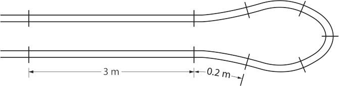
Figure 6 Suggested loop fastening - Replace any damaged loops entirely, or repair only if approved by the manufacturer.
- Maintain at least ¾″ of concrete over the top of tubing.
- Encase tubing that passes through an expansion joint inside a pipe sleeves that is one tube size larger.
- Pipe entering or exiting a concrete slab, or passing through an expansion joint, must do so through a sleeve.
- Tie tubing directly to WWF using twist ties or plastic straps. Make sure to cut off any ends that might protrude up through the top of the slab.
- Use enough ties to ensure the tubing won’t float upward during the pouring process. Maximum of 3m (10’) spacing between ties on a straight run, and 0.2m (8”) between ties on bends.
- Fill the system to 700 kPa (100 psi) for at least 30 minutes and inspect for leaks. Maintain water under pressure in the tubing while pouring concrete, to keep the tubes from floating.
- Once concrete pouring is finished, water pressure can be released from tubing. Blow out tubing using clean, dry air if freeze-up is possible.
- Do not re-pressurize tubing until concrete is up to its maximum pressure, in order to prevent the concrete from cracking.
Another important point to remember is to not store tubing in direct sunlight. UV rays are harmful to all plastics. Make sure that the tubing stays protected from the sun as long as possible before being installed.
Sizing the Heat Plant
Typically, boilers are the heat plant most commonly associated with hydronic heating, although with the increasing focus on green energy by the reduction of the use of fossil fuels, heat pumps are gaining in popularity. Regardless of the choice of heat plant used, the bottom line is that the heat plant’s output, not input, is the determining factor for sizing purposes. For example, if an estimate of a house’s heat loss were 37,841 btuh, then a boiler with an output of at least that amount would be needed. Also, one common rule of thumb is that the boiler’s output should be at least 10% greater than the estimated heat needed. However, there are others who maintain that a heat loss estimate is based on design conditions that aren’t very often encountered, and therefore the extra 10% output doesn’t necessarily need to be allowed for. In most cases, as long as a boiler’s output is greater than the heat load, there will likely be enough of a “buffer” there to deliver the heat needed even at the coldest times of the year.
Sizing the Circulator(s)
Sizing a circulator is not a straightforward task, and therefore many circulators in use are likely to have been chosen incorrectly for their application.
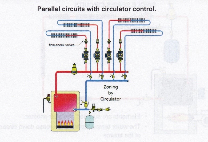
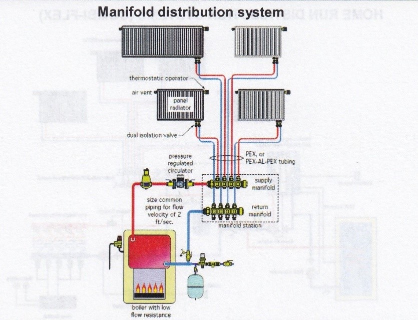
Firstly, the choice of piping strategy dictates how many circulators are needed and where they are to be located. Take for instance an old high-mass cast iron boiler feeding heat out through ¾″ copper tubing to baseboard convectors in a house. In most cases, a single circulator and multiple zone valves were used, and this “low head” system didn’t require the pump to produce much pressure, although it may have required a substantial flow rate in USGPM depending on the number of zones served. The pump should be installed downstream of the “point of no pressure change”. This is the point in the piping system where the expansion tank attaches to the supply main. The pump was chosen for its ability to move all the water in the system if all the zones were calling for heat, as well as to produce the pressure needed to overcome frictional losses through the piping, valves, fittings and any other component in the circuit with the highest head loss that the pump supplies.
It’s important to note that the head loss that a pump has to overcome is not the sum of the head losses through all the circuits that the pump supplies; it is only the single circuit with the most frictional resistance which includes the head loss through the longest loop that it supplies.
The illustration below is an example of lengths that must be considered when calculating the head against a pump.
The distance from the pump’s outlet to the most remote manifold or heat emitter and back to the pump’s inlet is measured, and an additional 50% of the measured length is added to reflect the extra frictional resistance caused by fittings and valves. This “equivalent” length is then converted into a head loss by using a table such as Table A on one of the pages that follow.
Secondly, today’s hydronic systems, with equipment such as heat exchangers and small diameter tubing, tend to have more head loss through their circuits than their “older” counterparts, which in turn requires a pump that produces more pressure. As well, if multiple pumps are used in place of zone valves, each one will have less water to move, and less frictional resistance that it has to overcome. So, the characteristics and requirements of circulators have changed with the times. Multiple small, high head, low flow rate pumps have largely replaced the single low head, high flow rate pumps found in the older, less sophisticated systems.
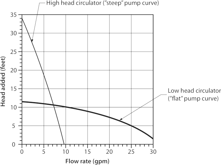
Pumps are chosen based on the two factors mentioned above, which are flow rate required (in USGPM) and resistance to flow that the pump must overcome (in feet of head). These two variables are able to be calculated and identified on a pump graph commonly known as a “pump curve”. The graphic below shows the performance curves for two pumps; one that produces a lot of pressure but not a lot of flow (high head) and the other that produces a lot of flow but not a lot of pressure (low head).

A pump will always deliver a certain flow based on the pressure it is offsetting. In the graph above, if the desired flow rate were to be 7 USGPM, or for simplicity from this point forward simply GPM, the low-head pump would be able to produce approximately 11 feet of head or about 4.8 psi. On the other hand, the high head pump, at 7 GPM flow rate, would produce approximately 15 feet of head or 6.5 psi. The system’s requirements therefore must be known before a pump can be selected. Just like a pump, the heating system has a “curve” which is a result of plotting the system requirements on a graph at varied flow rates. This is an involved process, so for ease of description we’ll be strictly dealing with a system’s maximum flow and head loss requirements so we can plot that single point on a pump graph.
The two widely accepted key points to remember when selecting a pump are:
- to avoid excessive pressure causing noise, choose the pump that has the “flattest” curve, and
- a pump’s curve must be “above” the system’s maximum requirements when plotted on the graph, in order to overcome the system’s head losses and still move enough water
Remember that the height of a closed system has no effect on a pump’s operation because it is a balanced system. Wherever the pump is located, the instant that the impeller starts to turn, water will want to move through the system to re-enter the pump’s intake port. So, if a pump doesn’t have to overcome pressure created by a system’s height, the only thing it has to overcome is the frictional resistance of the system components. In order to be able to correctly identify those friction losses, we have to first know the flow rates.
Calculating Flow Rates
The heat that we’re trying to supply is expressed in BTUH, but to deliver that within a hydronic system using a pump, we need to turn BTUH (herat loss language) into GPM (pump language). The formula to use is:
BTUH ÷ 10,000 = GPM
This divisor of 10,000 is arrived at by multiplying 20°ΔT (industry-standard temperature differential) × 60 (minutes per hour) × 8.33 (pounds per USG)
The number is actually 9,996 BTUH per USGPM, but for the sake of 4 BTUH we can use 10,000 so that the calculation can usually be performed in one’s head. So, if a pump had to deliver 64,325 BTUH at a ΔT of 20°F it would have to move at least 6.4 GPM. Some designers may choose to use a different ΔT for their systems. The flow rate divisor used would then be calculated as ΔT × 60 × 8.33. A ΔT of 15°F would use a divisor of 7,497 (7,500) BTUH per USGPM. For a 15°FΔT our heat requirement example above would need a flow rate of 64,325 BTUH ÷ 7,500 = 8.4 USGPM. A 10°ΔT would use a divisor of 5,000 BTUH per USGPM and so on. Because the industry has used a 20°FΔT for decades, we will always assume a divisor of 10,000.
Calculating Friction Losses
In order to calculate friction loss for any given piping circuit, designers not only have to know the expected flow rate through it (see above), they also need to know the components that the water will have to go through within that circuit. We know by now that frictional losses will increase if the flow rate increases – Bernoulli told us so. High flow rates in GPM will cause high frictional losses. In hot water heating systems, the idea is to keep flow rates low, somewhere between 1 and 4 feet per second, so that frictional losses can be held to a minimum. If water were moved very quickly through a system, not only would there be increased noise and erosion but there would be less time to let the heat that it contains be transferred to the heat transfer units. Tables have been created for hydronics designers that corelate a desired limit of frictional resistance with an equivalent length of piping. In domestic potable water systems where water moves very fast and at high pressures, friction loss is expressed as PSI/foot or feet of head/foot. For hydronic heating systems, the frictional resistance expression needs smaller units known as millinches per foot. A foot contains 12 inches and, instead of eighths, sixteenths or sixty-fourths, each inch is split into 1,000 parts called millinches. Translated into frictional losses of PSI per foot, 1 millinch/foot would be equivalent to 0.000083 psi per foot. The norm for designers is to move water through a system so that the frictional losses are kept to somewhere between 100 and 500 millinches per foot, with 400 millinches/foot being the design norm.
The table shown below equates an equivalent length of pipe to a frictional loss for that length, at head losses between 200 and 500 millinches per foot.
| Pressure Head of Feet | Piping Friction Loss — Millinches per Ft of pipe | |||||
|---|---|---|---|---|---|---|
| 500 | 400 | 350 | 300 | 250 | 200 | |
| 2 | 48 | 60 | 69 | 80 | 96 | 120 |
| 2.5 | 60 | 75 | 84 | 100 | 120 | 150 |
| 3 | 72 | 90 | 102 | 120 | 144 | 180 |
| 3.5 | 84 | 105 | 120 | 140 | 168 | 210 |
| 4 | 96 | 120 | 137 | 160 | 192 | 240 |
| 4.5 | 108 | 135 | 154 | 180 | 216 | 270 |
| 5 | 120 | 150 | 171 | 200 | 240 | 300 |
| 5.5 | 132 | 165 | 188 | 220 | 264 | 330 |
| 6 | 144 | 180 | 206 | 240 | 288 | 360 |
| 6.5 | 156 | 195 | 223 | 260 | 312 | 390 |
| 7 | 168 | 210 | 240 | 280 | 336 | 420 |
| 7.5 | 180 | 225 | 256 | 300 | 360 | 450 |
| 8 | 192 | 240 | 274 | 320 | 384 | 480 |
| 8.5 | 204 | 255 | 292 | 340 | 408 | 510 |
| 9 | 216 | 270 | 309 | 360 | 432 | 540 |
| 9.5 | 228 | 285 | 326 | 380 | 456 | 570 |
| 10 | 240 | 300 | 343 | 400 | 480 | 600 |
| 10.5 | 252 | 315 | 360 | 420 | 504 | 630 |
| 11 | 264 | 330 | 376 | 440 | 528 | 660 |
| 11.5 | 276 | 345 | 395 | 460 | 552 | 690 |
| 12 | 288 | 360 | 410 | 480 | 576 | 720 |
| 15 | 360 | 450 | 515 | 600 | 720 | 900 |
| 20 | 480 | 600 | 686 | 800 | 960 | 1200 |
| 25 | 600 | 750 | 857 | 1000 | 1200 | 1500 |
| 30 | 720 | 900 | 1030 | 1200 | 1440 | 1800 |
| 35 | 840 | 1050 | 1200 | 1400 | 1680 | 2100 |
| 40 | 960 | 1200 | 1370 | 1600 | 1920 | 2400 |
| 50 | 1200 | 1500 | 1725 | 2000 | 2400 | 3000 |
Equivalent length means taking the actual measured length and adding 50% to it to simulate extra losses through fittings. For example, a measured length of 70 feet, from outlet of the pump around through the circuit it serves and back to the inlet, would be considered to be 70 × 1.5 = 105 equivalent feet. As you can see, the shaded area on the table represents 400 millinches/ft. (the desired limit). Reading down that shaded column, we see that an equivalent length of pipe of 105 feet would be considered to have a head loss of 3.5 feet of head pressure against the pump. 150 feet of pipe at 400 millinches/ft would be given a total head loss of 5 feet, and so on. The units of measure can always be translated back and forth between feet of head and psi by using the .433 multiplier or its inverse of 2.31, but pump language for pressure is in feet of head.
Loop Losses
The table shown above is meant to assign a head loss to the supply and return piping near the boiler and out to the manifolds. Additionally, the head loss through the longest loop supplied by a manifold will have to be determined so it can be added to the other heads that the pump must overcome. Manufacturers of PeX tubing publish the head losses for their various types and sizes of tube, at different flow rates and temperatures and with different glycol mixtures. Because the tubing from various manufacturers is consistent in its inside diameter, tables from different manufacturers will be all but identical and their results are similar enough to be relied upon. Below is a table for the head loss through 100 feet of ½″ PeX “A” tubing using 100% water (no glycol).
| gpm | Velocity (ft/s) |
40°F 4°C |
60°F 16°C |
80°F 27°C |
100°F 38°C |
120°F 49°C |
140°F 60°C |
160°F 71°C |
180°F 82°C |
|---|---|---|---|---|---|---|---|---|---|
| 0.1 | 0.18 | 0.06 | 0.05 | 0.05 | 0.05 | 0.05 | 0.05 | 0.04 | 0.04 |
| 0.2 | 0.36 | 0.21 | 0.19 | 0.18 | 0.18 | 0.17 | 0.16 | 0.16 | 0.16 |
| 0.3 | 0.54 | 0.44 | 0.41 | 0.39 | 0.37 | 0.36 | 0.35 | 0.34 | 0.33 |
| 0.4 | 0.72 | 0.75 | 0.70 | 0.66 | 0.64 | 0.61 | 0.59 | 0.58 | 0.57 |
| 0.5 | 0.91 | 1.14 | 1.05 | 1.00 | 0.96 | 0.92 | 0.89 | 0.88 | 0.86 |
| 0.6 | 1.09 | 1.59 | 1.47 | 1.40 | 1.35 | 1.29 | 1.25 | 1.23 | 1.20 |
| 0.7 | 1.27 | 2.12 | 1.96 | 1.86 | 1.79 | 1.71 | 1.66 | 1.63 | 1.60 |
| 0.8 | 1.45 | 2.72 | 2.51 | 2.38 | 2.30 | 2.19 | 2.13 | 2.09 | 2.05 |
| 0.9 | 1.63 | 3.38 | 3.12 | 2.96 | 2.86 | 2.73 | 2.65 | 2.60 | 2.55 |
| 1.0 | 1.81 | 4.10 | 3.79 | 3.60 | 3.47 | 3.31 | 3.22 | 3.16 | 3.09 |
To arrive at a head loss for a loop, simply find the closest temperature and flow rate for the desired loop, and adjust the table’s head loss to reflect the actual loop length. For instance, for a loop that operates at 118°F and .65 GPM, enter the table by choosing 100°F and 0.7 GPM, which would be 1.79 feet of head per 100 feet of tubing. The rationale here is that colder water will have more frictional resistance than hot water, and 0.70 GPM will be more restrictive than 0.60 GPM. This approach will ensure that the pump will be able to move the water at the actual temperatures and flow rates. Once the head loss is identified from the table, multiply that number by the actual length of the loop. For the example above, if the loop’s actual length was 240 feet, then the head loss through it would be 2.4 × 1.79 = 4.3 feet of head.
The Effects of Glycol
Winters in Canada can be very cold, depending on location, and in rural areas a constant electrical power supply can be hit-and-miss, so an antifreeze solution, rather than 100% water, may be a good choice for a hydronic system. However, there are effects that must be considered.
Firstly, there must be an acceptable backflow prevention device installed on the cold water makeup to the system. Where a “dual check with atmospheric port” (DCAP) device is the norm as a backflow preventer for residential systems that are not more than 250,000 btuh of input and have no chemicals added, a reduced pressure backflow assembly (RPBA) will be needed once any chemicals of any kind are added.
Secondly, the appropriate type of glycol to be used is polypropylene glycol, which is known as food-grade antifreeze. It is non-toxic but expensive. It’s counterpart, ethylene glycol, is used in the automotive industry, and although less expensive than polypropylene glycol, it is extremely toxic, and its use in a hydronic system that is directly connected to a potable water supply is strongly discouraged, with or without backflow prevention.
Thirdly, glycol will have an effect on pumps and expansion tanks. The chart below illustrates the increase in effort that will be put on pumps that are trying to move a thicker-than-water solution. Depending on the temperature (hot water is “thinner” than cold water), a 50% glycol/water solution will be anywhere from 14% to 22% harder to move, and will create more head pressure as well, up to 2.14 times that which 100% water would create at 40°F
| Fluid Temperature °F | % Adjustment Factor |
|---|---|
| 40°F | 1.22 |
| 100°F | 1.16 |
| 140°F | 1.15 |
| 180°F | 1.14 |
| 220°F | 1.14 |
| Fluid Temperature °F | % Adjustment Factor |
|---|---|
| 40°F | 2.14 |
| 100°F | 1.49 |
| 140°F | 1.32 |
| 180°F | 1.23 |
| 220°F | 1.18 |
Lastly, any glycol will have a detrimental effect on any rubber components in the system, mainly the rubber ball inside a zone valve. Over time, the rubber will erode and eventually disintegrate.
In summary, the use of glycol should be avoided if at all possible.
Another variable that must be known will be the use of any specialty components on a pump’s circuit. These are circuit balancing valves (known as “circuit setters”), mixing valves and heat exchangers.
Circuit Balancing Valves (“Circuit Setters”)
A pump will move water at a certain flow rate depending on the head losses that it is pumping against. If the flow rate through a circuit needs to be as accurate as possible, a balancing valve may have to be installed. They are a low-loss type of globe valve, and will have ports known as “Pete’s Plugs” on the upstream and downstream sides of the valve seat. “Pete” is a twist of the expression “PT” which stands for pressure/temperature.
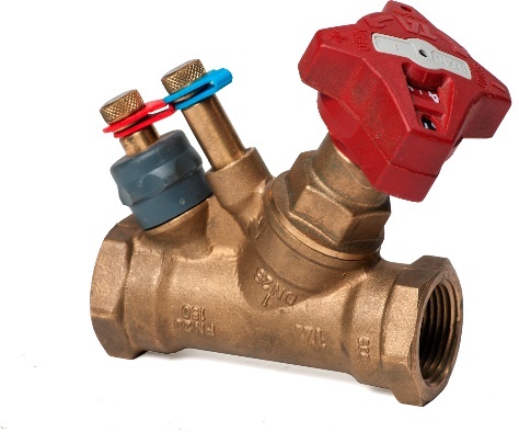
Flow rate is measured by attaching a differential pressure gauge to the Pete’s plugs and reading the ΔP across the valve. This reading is applied to a table for that particular valve which will indicate the GPM through the it at that setting. Adjusting the valve will alter the ΔP across it and thereby the flow rate.
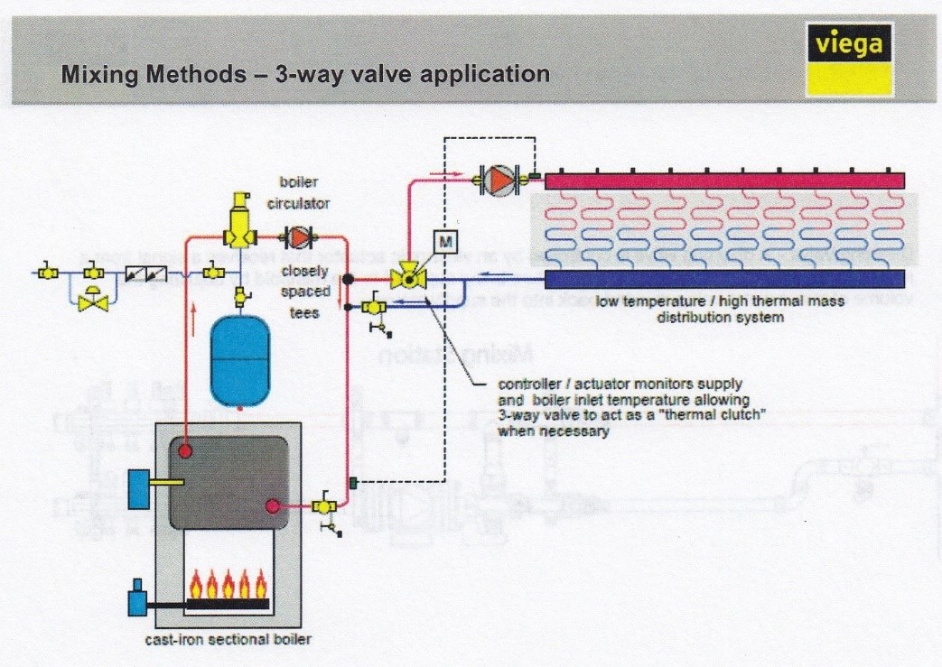
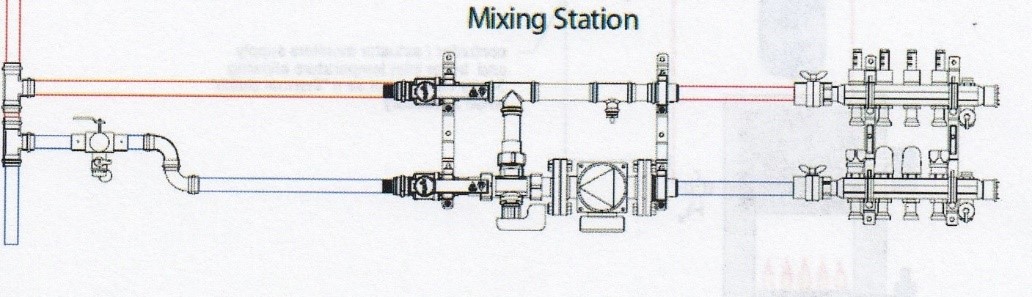
Tempering Valves
If a system requires water temperatures that differ greatly, such as when a non-condensing boiler has to feed a radiant floor panel, the water to the panel must be tempered, and there are different valves available that can be used. They come in various types, configurations and sizes, and as such may be located in different points in the system.
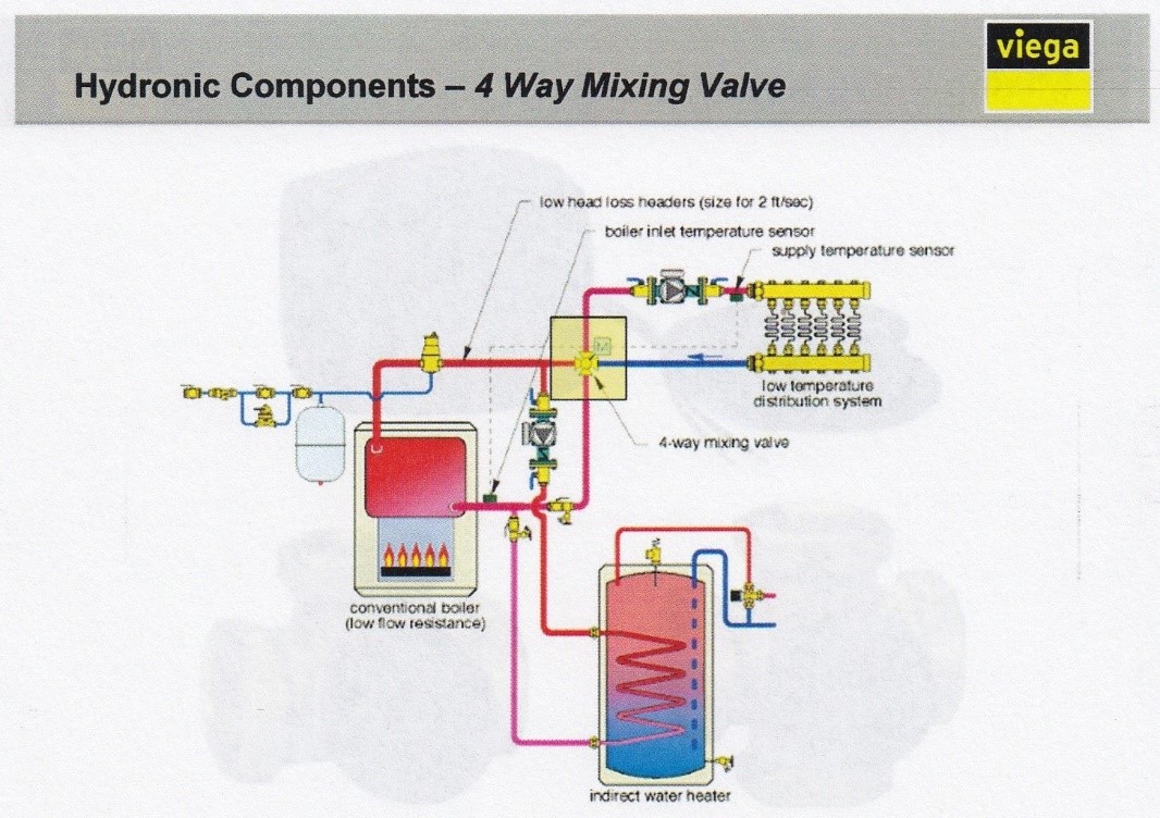
Mixing Valves
A mixing valve can have either 2, 3 or 4 ports and is located at the point where high temperature water from the boiler and some of the low temperature return water converge, known as the “mixing point”, with the tempered water going out to the system and the remainder of the return water going back to the boiler. Some examples of 3-way and 4-way mixing valves are shown below.
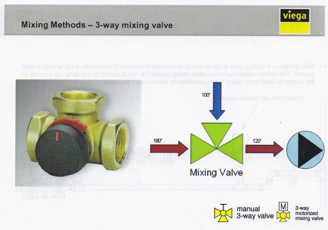
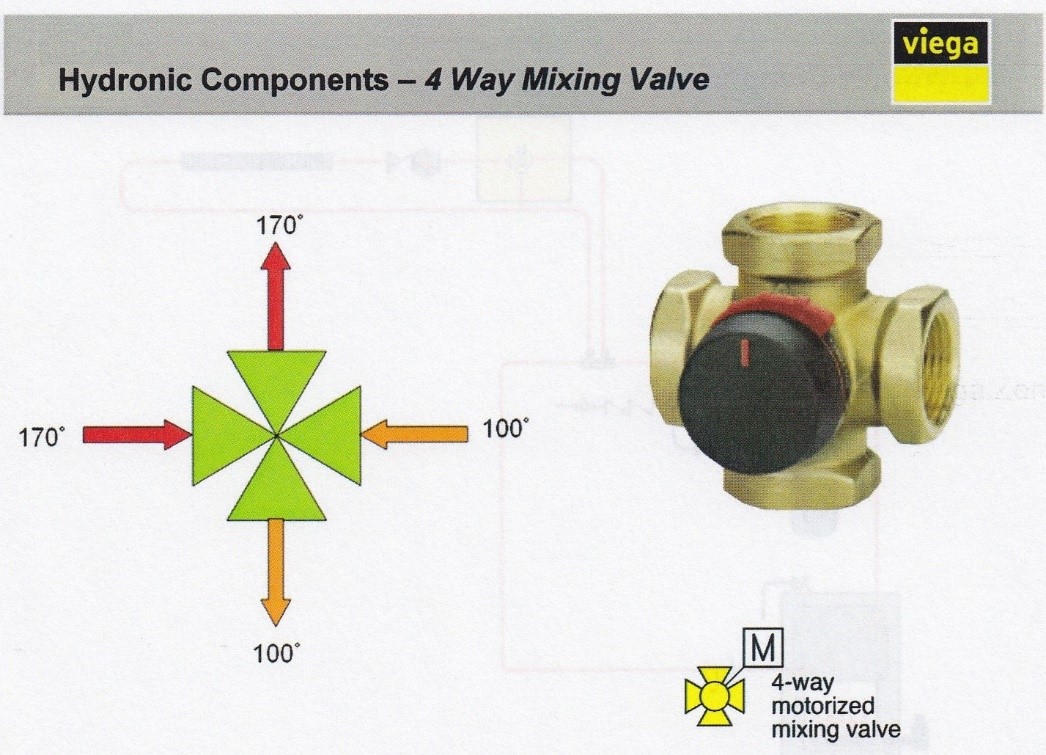
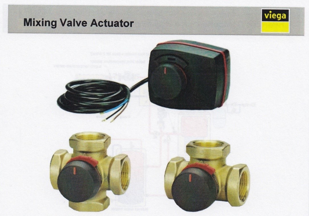
The mixing valves can either be manually pre-set to supply a constant temperature (known as thermostatic) or can have a motorized actuator and controller added which is capable of modulating the temperatures as thermal conditions change (known as reset control).
Diverting Valves
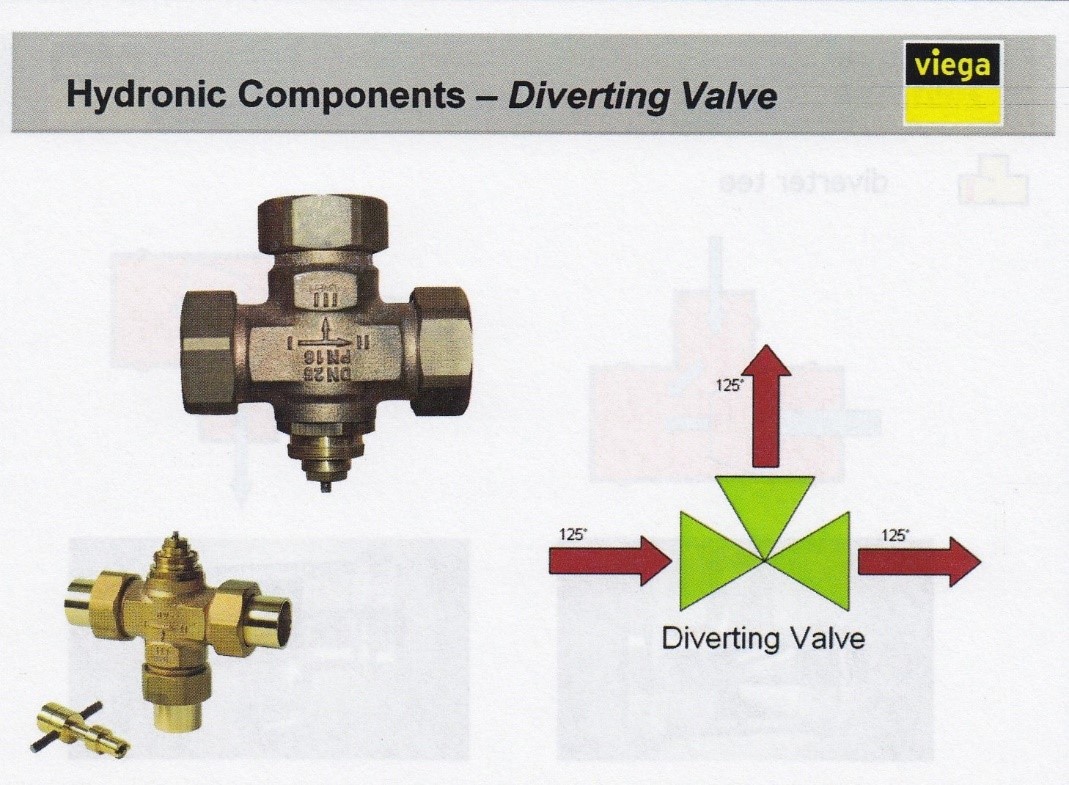
There are a few differences between a diverting valve and a mixing valve. Diverting valves have the same entering and leaving water temperatures, and so are not located at the mixing point; rather it is located on the return piping, as seen in the diagram below.
There is more explanation of these valves in a later module.
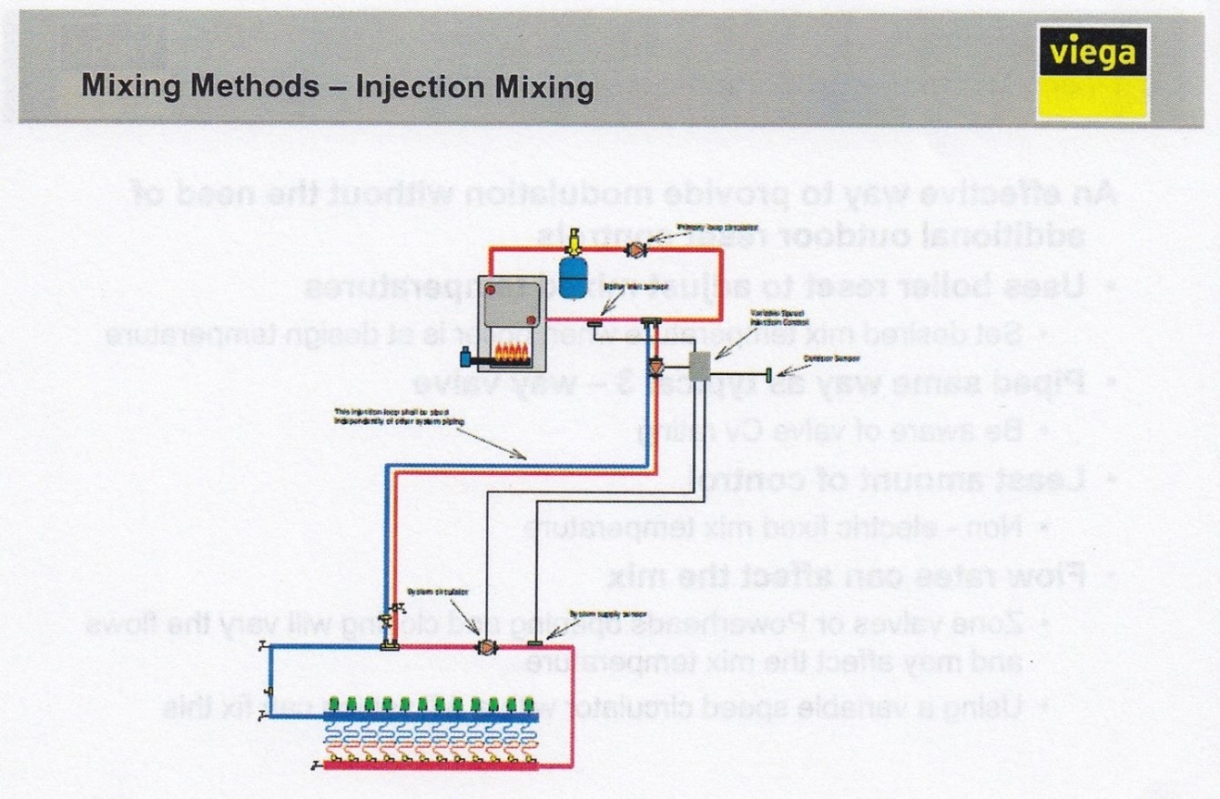
Injection Mixing
Another popular strategy for adjusting mixed water temperatures to manifolds is through the use of a pump to “inject” an amount of hot water into the supply side of a manifold, appropriately called “injection mixing”. Injection pumps are commonly used in conjunction with primary-secondary piping systems. A temperature controller reacts to a sensor’s output and sends a signal to a pump that the supply loop needs heat. The variable-speed pump sets itself to the speed required in order to maintain a desired temperature.
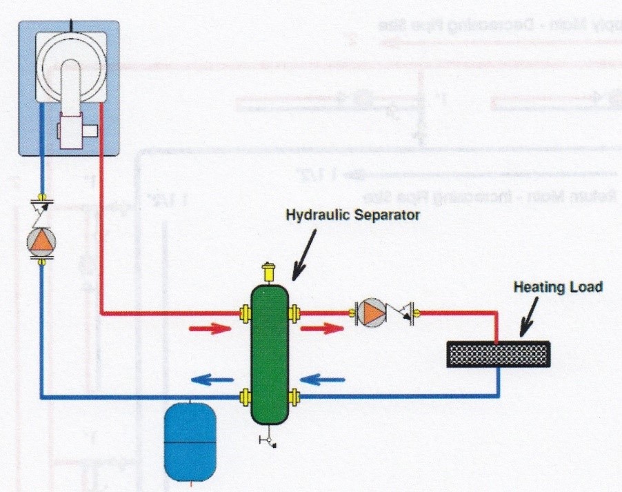
Hydraulic Separation
Multiple pumps which share piping must be hydraulically separated from each other to ensure that the operation of one pump can’t affect the operation of the other. This can be accomplished by using a “hydraulic separator”, which can be as simple as a tank or large vessel that has very low head loss through it.
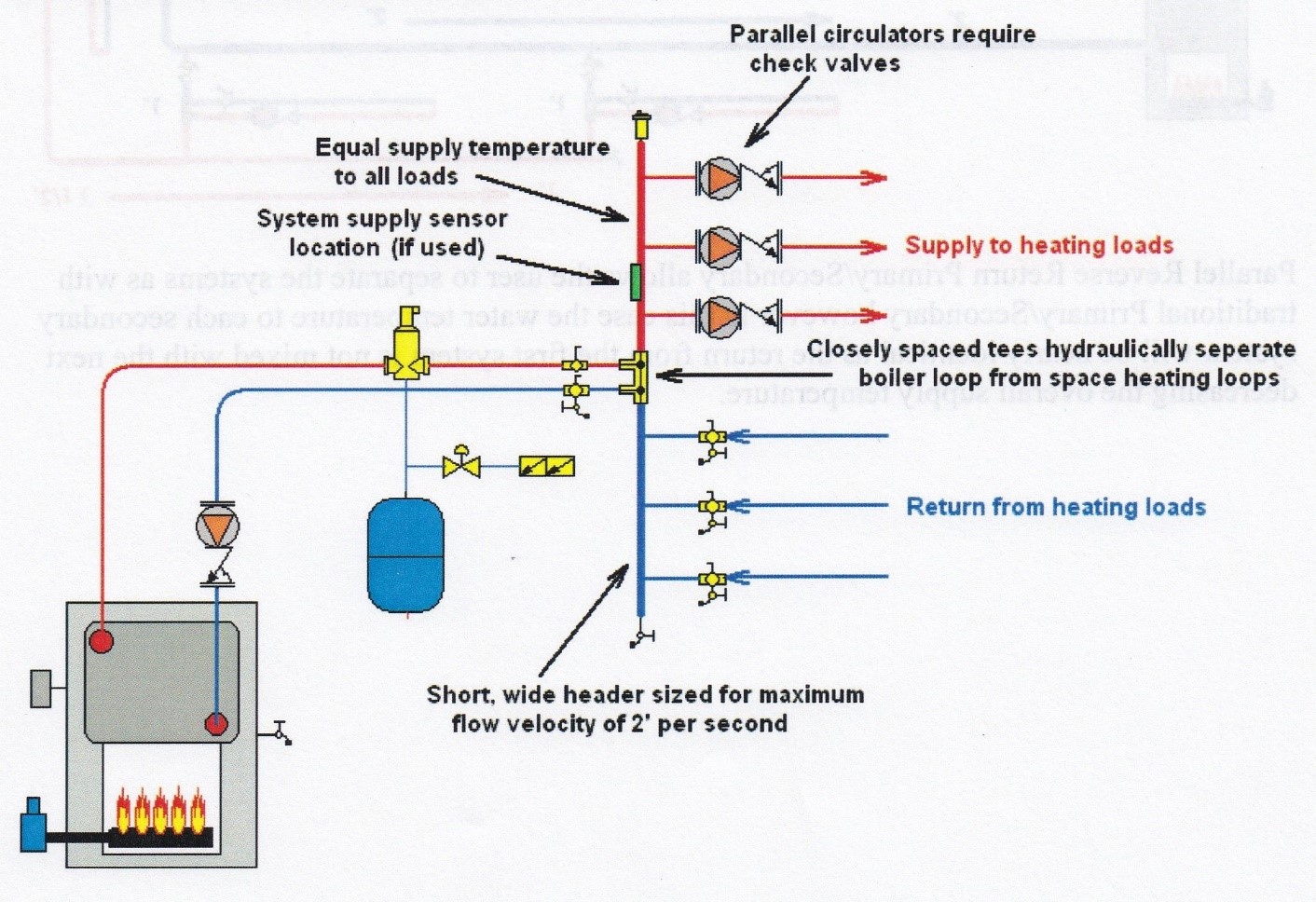
This separation can also be through the use of tees located very close to one another as in the graphic below.
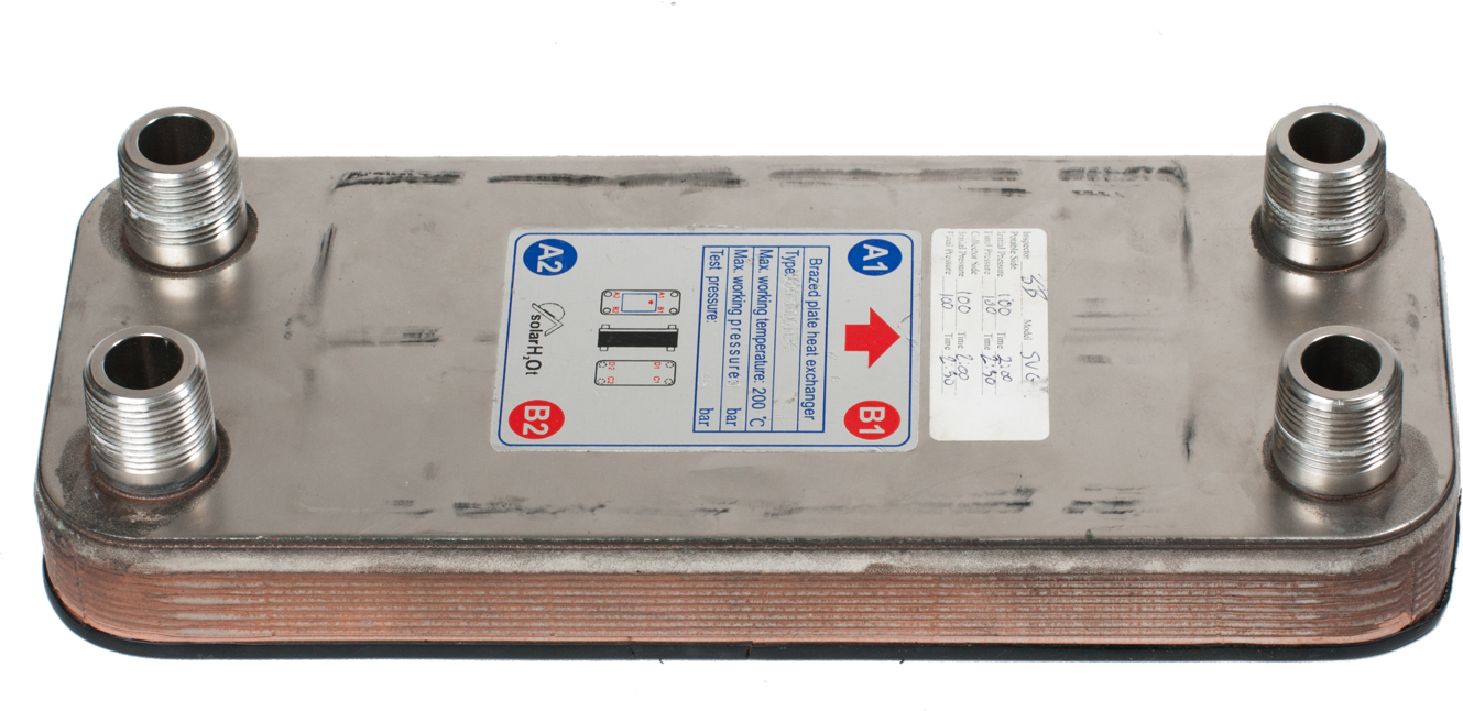
Heat Exchangers
Brazed plate heat exchangers used in residential and small commercial systems are very compact but have enormous heat exchange capacities. This is because the small spaces between the stainless-steel plates inside them have a huge surface area. Consequently, pumps have to work harder than normal to push water through them.
CV Value
The manufacturers of high head loss components, such as mixing valves and heat exchangers, assign numbers to them for use in head loss calculations, known as “CV” (control valve) values. A CV value is the flow rate in GPM through the valve that would result in a 1 psi pressure drop across it. The same valve used in two different piping systems will have differing head losses through it because of the existence of differing flow rates. To calculate the pressure drop through a valve at a specific flow rate, use the following formulaΔP = (Q ÷ CV)² where Q = desired flow rate and ΔP is the pressure drop in PSI.
As an example, let’s say that we are intending to use a valve that has a CV rating of 2.5. This means at a flow rate of 2.5 GPM, the pressure drop across the valve will be 1 psi. If we need to know what the pressure drop across the valve will be at a flow rate of 3.2 GPM, we would calculate it as follows:
ΔP = (3.2 ÷ 2.5)² = 1.64 PSI which translates to 3.79 feet of head.
To correctly size a pump, the total head losses for the piping and devices that it must push water through are applied to the vertical axis (left side) of a pump graph. Draw a horizontal line across the graph from that point, then find the desired flow rate in GPM that it must supply along the horizontal axis at the bottom of the page and draw a vertical line upward through the graph from that point. The intersection of the horizontal and vertical lines would be the maximum needs of the system in head loss and flow rate, called the “system operating point”. For a pump to be effective, its curve has to fall above the system operating point. If it isn’t, it won’t put out enough pressure at the required flow rate to offset the frictional losses.
Looking at the chart above, if a system’s operating point was 15 feet of head @ 5 GPM, the pump with the flat curve would only create 11 feet of head pressure at 5 GPM, and so would not do the job. The pump with the steep curve would put out approximately 18 feet of head pressure while moving 5 GPM and would work for that application. The ideal pump chosen would be one with a “flat” curve so as to avoid excessive pressure which creates noisy systems. As well, whenever possible, select circulators so that the operating point of the system falls within the middle third of their pump curve. This is the region where the circulator’s efficiency is relatively high.
Some points to remember when installing pumps are:
- Many modern pumps are capable of operating at three different speeds. When using this variety of pump, always select the lowest speed that will deliver the head and flow rate required.
- Always locate circulators so that the connecting point of the system’s expansion tank (“point of no pressure change”) is as near the inlet of the circulator(s) as possible. This allows the circulator to “pump away” from the point of no pressure change and thereby increase the pressure in the circuit.
- Always provide hydraulic separation between any circulators in a system that could operate simultaneously. This prevents interference between the circulators, especially when they have very different flow/head ratings.
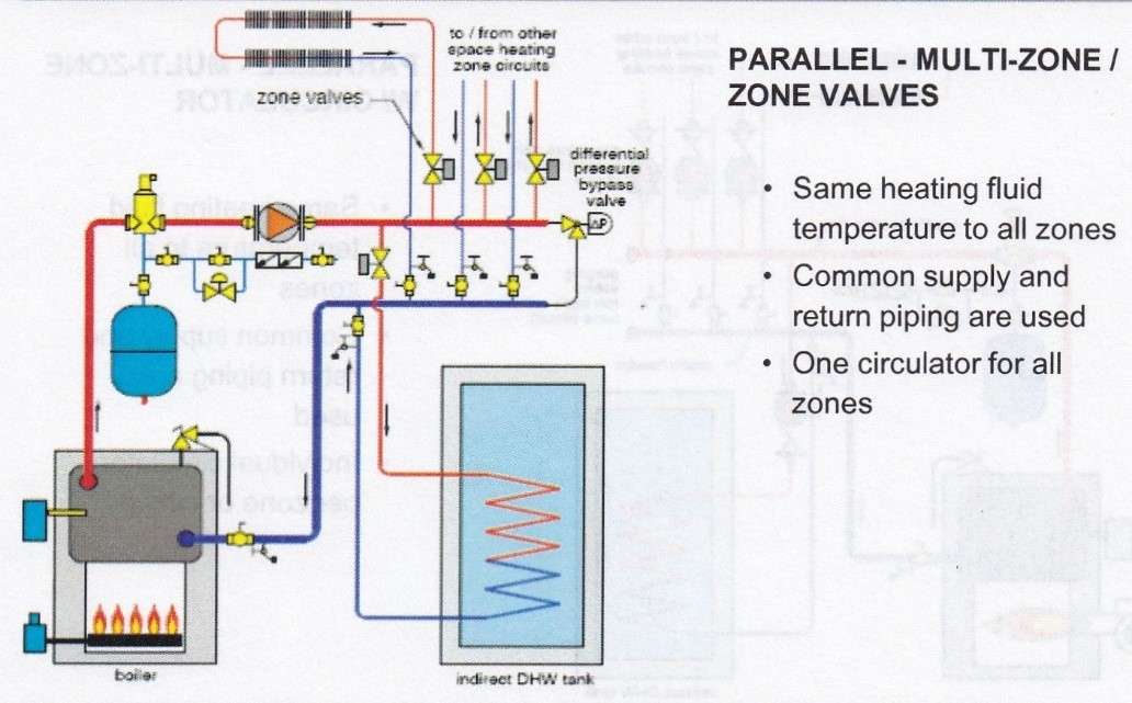
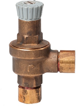
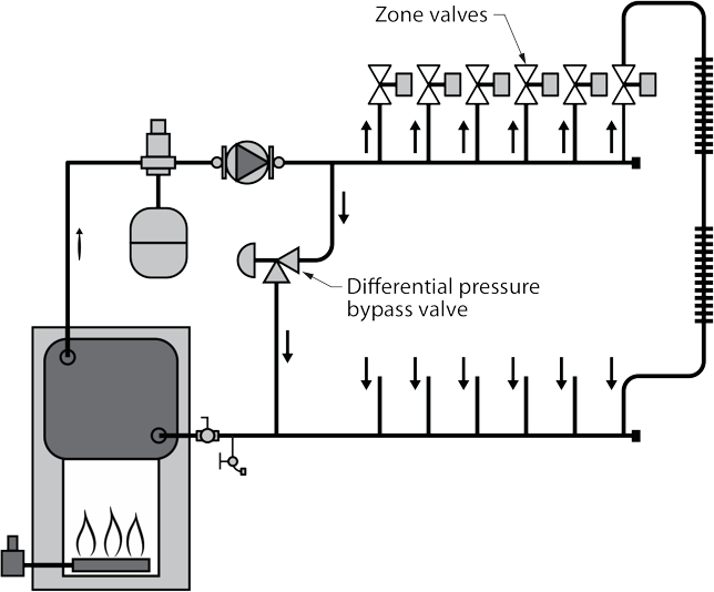
For systems using a single pump and multiple zone valves, a differential pressure valve (DPV) is usually installed to avoid over-pressurizing the system in situations where there are only one or two zones calling for heat. A DPV will open to bypass water from the supply main to the return main when excessive pressure is sensed.
Another way of regulating differential pressure in hydronic systems is through use of variable-speed circulators. This method has been used in larger hydronic systems for several years. It is accomplished through the use of electronic pressure transducers that communicate to a variable frequency drive (VFD) to electrically adjust the speed of an AC circulator motor. The more recent availability of smaller circulators with electronically commutated motors (ECM) now makes similar control techniques available in smaller residential hydronic heating and cooling systems. These “pressure-regulated” ECM circulators are ideal for systems using valve-based zoning. They eliminate the need for a differential pressure bypass valve. They also eliminate the need of pressure transducers and variable frequency drives.
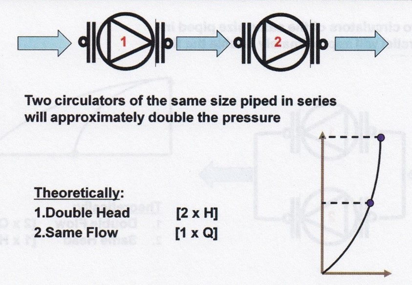
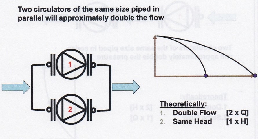
Designers will sometimes specify circulators installed in series or in parallel with each other in the same piping circuit. Two pumps in series with each other will roughly double the pressure output while the flow rate will roughly remain unchanged, while two circulators in parallel will roughly double the flow rate while not appreciably affecting the output pressure.
Installing two small circulators, rather than one large one, has proven cost-effective. For more in-depth information on circulators, visit websites such as caleffi.com, tacocomfort.com and Grundfos.com among others.
Sizing Expansion Tanks
Expansion tanks, also known as cushion or compression tanks, keep the system pressure from fluctuating widely when the system water heats up and cools down. Without one, the pressure buildup caused by thermal expansion would trip the pressure relief valve and discharge enough system water to keep the pressure at that maximum level. Once the boiler shuts off and the system water cools, the pressure will now drop below the fill valve’s setpoint and enough water will be added to hold the desired setpoint pressure. This sequence will repeat every time the boiler cycles on and off. The constant addition of fresh water to the system will eventually lead to rusting of ferrous components such as circulators and boilers, and leaks in these components would indicate that the system is in dire need of repair or replacement. Expansion tanks that are properly sized and maintained prevent all this from occurring.
Correctly sizing an expansion tank involves knowing:
- the minimum and maximum operating pressures
- the system volume in gallons
- the minimum and maximum operating temperatures, and
- the percentage mixture of glycol (if applicable)
Just as in pump sizing, manufacturers of expansion tanks publish sizing literature and tables to assist in the process. These are based on formulas that, for non-engineers, are much too complex and time consuming for most to deal with.
The old “conventional” expansion tanks were simply closed tanks where water and air were in direct contact with each other. Over time, air is re-absorbed into the water, which reduces the air volume until the tank has so little air that it is, for all intents and purposes, non-existent. The tank at this point is called “waterlogged” and will cause the aforementioned cycle of discharging/adding water.
Diaphragm-type tanks are the norm today.
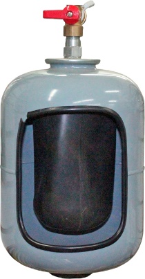
As long as there is a butyl rubber or EPDM membrane separating the water and air, the waterlogging issues are largely a thing of the past. These newer styles of tanks can be smaller because of the pre-set air charge within them, and because system water isn’t in direct contact with the steel of the tank, corrosion of the tank is greatly reduced. A diaphragm tank that shows water leaking from pinholes in the shell is an indicator that the rubber membrane has failed and that fresh water being repeatedly admitted into the system is causing corrosion. Fortunately, the thinnest steel in the entire system is in the shell of the diaphragm expansion tank, and corrosion problems within the system, evidenced by these pinholes, can usually be caught early enough to avoid a lot of damage to the major components.
A properly-sized diaphragm-type expansion tank should reach a maximum pressure about 5 psi lower than the relief valve setting when the system pressure reaches its maximum operating temperature. This prevents the relief valve from leaking at pressures just below its rated opening pressure.
The first step in sizing a diaphragm-type expansion tank is to determine the proper air-side pressurization of the tank using the following equation;
Pa = (H × .433) + 5 where;
- “Pa” is the air-side pressurization of the tank in psi
- “H” is the height from the inlet of the expansion tank to the top of the system in feet
- “.433” is the density of water at its unheated temperature per foot of height, and
- “5” is the desired pressure to maintain at the top of the system in PSI.
For example, if the top of the piping circuit was 25 feet above the expansion tank connection and assuming the system is filled with water, the correct air side pressure in the tank would be calculated as:
Pa = (25 × .433) + 5Pa = (25 × .433) + 5Pa = 10.83 + 5Pa = 15.83 psi
As you can see from the equation above, the correct set pressure for both the system fill valve and the air fill pressure for the tank is not simply 12 or 15 psi as is most commonly thought. The height of the system has to be factored in to be able to set these pressures correctly.
The pressure on the air-side of the diaphragm should be adjusted to this value before fluid is added to the system. Proper air-side pressure adjustment ensures the diaphragm will be fully expanded against the shell of the tank when the system is filled with fluid, but before it is heated. Failure to make this adjustment can result in the diaphragm being partially compressed before any heating occurs, and the full expansion volume of the tank would not be available as the fluid heats up. An underpressurized tank will act as if undersized, and possibly cause the relief valve to open each time the system heats up. This situation must be avoided. Use a low-pressure type of tire gauge with a scale of 0-30 psi and a bicycle pump or small air compressor to set the calculated air side pressure before filling the system with fluid.
The next step is to determine the volume of water in the system. This is also a fairly drawn-out endeavour if attempting to do long-hand, which involves measuring and calculating the volume of all the different piping by size and length, as well as the volume within the boiler and heat transfer units. Instead, various expansion tank manufacturers and hydronics partners have come up with shortcut methods that are very accurate when used in residential systems. One such method is given in TECA’s “Hydronic System Design” manual, which uses a combination of heat emitter types and heat load from a table (shown below) and applies these values to a step-by-step process in the worksheet also shown below. This results in an “acceptance volume” which is the volume, in gallons, that an expansion tank has to be able to allow to come into it when the system water heats up and expands in volume.
| Gal | Litre | Base Board Heater
6 l/kW 4.65 USG/1000 BTU 195°F (90°C) |
Panel Radiator
8.33 l/kW 6.45 USG/1000 BTU 195°F (90°C) |
Cast Iron Radiator
12 l/kW 9.3 USG/1000 BTU 195°F (90°C) |
Steel Radiator
15 l/kW 11.6 USG/1000 BTU 195°F (90°C) |
Floor Htg
18.5 l/kW ¾″ ID Tube 122°F (50°C) |
Floor Htg
9.29 USG/1000 BTU ½″ ID Tube 122°F (50°C) |
|---|---|---|---|---|---|---|---|
| 0.5 | 2 | 16,036 | 11,600 | 7,847 | 6,482 | 14,625 | 22,420 |
| 1 | 4 | 32,072 | 23,201 | 16,036 | 12,965 | 29,245 | 45,817 |
| 2 | 8 | 64,145 | 46,062 | 32,072 | 25,590 | 59,500 | 91,634 |
| 3 | 12 | 96,263 | 69,263 | 48,109 | 38,555 | 88,710 | 137,450 |
| 4.8 | 18 | 144,327 | 103,724 | 71,993 | 57,622 | 133,550 | 205,700 |
| 6.6 | 25 | 200,284 | 144,327 | 99,971 | 80,182 | 185,200 | 285,600 |
| 9 | 35 | 280,466 | 201,990 | 140,233 | 112,254 | 260,000 | 400,000 |
| 13 | 50 | 399,204 | 288,314 | 200,284 | 160,022 | 371,400 | 572,240 |
| 21 | 80 | 641,456 | 460,620 | 318,680 | 256,241 | 590,000 | 910,500 |
| 29 | 110 | 880,296 | 634,632 | 440,148 | 351,436 | 816,000 | 1,257,500 |
| 37 | 140 | 1,122,548 | 808,644 | 559,569 | 446,972 | 1,043,000 | 1,598,700 |
Heat Capacity in BTUH with a max. operating pressure of 30 psi.
Note: To Calculate Acceptance Volume of BTUH not listed on Table 2.5:
[latex]\dfrac{\text{Unlisted BTUH}}{\text{next Listed BTUH}}=\underline{\qquad} \times \text{Acc. Volume for next listed BTUH}=\text{Acceptance Volume for unlisted BTUH}[/latex]
Example: For an unlisted BTUH OF 24,054
[latex]24,054 \div 32,072 = \underline{.75} \times 1\text{ gal} = .75 \text{ Gallon Acceptance Volume for 24,054 BTUH}[/latex]
Quick Method - Expansion Tank Sizing by Heat Capacity[2]
This method is based on standard residential heating systems and piping capacities. It is very accurate for typical residential installations and may be used with confidence for sizing such systems.
- Step 1: Type of heating system (or combination): Record BTUH from Heat Loss Worksheet.
- Step 2: Acceptance Volume: Use Table 2.5. If BTUH value other than listed, calculate acceptance volume as shown in Table Note.
- Step 3: Acceptance Volume Adjustment for temperature: If temperature other than listed in Table 2.5, enter Factor from Table 2.6a or 2.6b.
- Step 4: Total System Acceptance Volume. Record adjusted Acceptance Volume(s) and total in Box G.
[latex]\begin{array}{llccccc} &\text{Step 1}&\text{Step 2}&&\text{Step3}&&\text{Step 4}\\ &\text{BTUH}&\text{Acc Volume}&&\text{Temp Factor}&&\text{Adj Acc Volume}\\ 1.\text{Base Board}& \underline{\qquad} \text{BTU} & \underline{\qquad}& \times &\underline{\qquad}&=&\underline{\qquad} \text{Gal(L)}\textbf{A}\\ 2.\text{Panel Radiator}& \underline{\qquad} \text{BTU} & \underline{\qquad}& \times &\underline{\qquad}&=&\underline{\qquad} \text{Gal(L)}\textbf{B}\\ 3.\text{Cast Iron Radiator}& \underline{\qquad} \text{BTU} & \underline{\qquad}& \times &\underline{\qquad}&=&\underline{\qquad} \text{Gal(L)}\textbf{C}\\ 4.\text{Steel Radiator}& \underline{\qquad} \text{BTU} & \underline{\qquad}& \times &\underline{\qquad}&=&\underline{\qquad} \text{Gal(L)}\textbf{D}\\ 5.\text{Floor Heating ¾″}& \underline{\qquad} \text{BTU} & \underline{\qquad}& \times &\underline{\qquad}&=&\underline{\qquad} \text{Gal(L)}\textbf{E}\\ 6.\text{Floor Heating ½″}& \underline{\qquad} \text{BTU} & \underline{\qquad}& \times &\underline{\qquad}&=&\underline{\qquad} \text{Gal(L)}\textbf{F}\\ \end{array}[/latex]
[latex]\text{Total Acceptance Volume (Add Value A through F as required)}=\underline{\qquad}\text{Gal{L}}\textbf{G}[/latex] - Step 5: If Glycol is added to the system use Table 2.7.
[latex]\dfrac{\qquad}{\text{Value G}}\times \dfrac{\qquad}{\text{Corr. Factor}}=\text{Acceptance value adjusted for Glycol in system}=\underline{\qquad}\textbf{ H}[/latex]
Table 2.5 above has an assumed temperature of 195°F for four of the listed systems, and 122°F for the other two. If the system’s temperature is otherwise, an adjustment is made by the use of a temperature adjustment factor, shown in Table 2.6a and 2.6b below, that is used as a multiplier in the worksheet.
| Temp | Factor |
|---|---|
| 140°F/60°C | 0.47 |
| 158°F/70°C | 0.61 |
| 176°F/80°C | 0.81 |
| 212°F/100°C | 1.21 |
| Temp | Factor |
|---|---|
| 104°F/40°C | 0.77 |
| 122°F/50°C | 1.00 |
| 140°F/60°C | 1.34 |
| 158°F/70°C | 1.74 |
Lastly, an extra allowance must be made if the system will have glycol for freeze protection. The table below lists factors to be applied and sets out recommended water/glycol percentage mixtures dependent upon outdoor temperatures.
| Outdoor Temp | % Glycol to be added to heating water | Water Glycol Mix expansion from freeze temperature up to 194°F (90°C) | Expansion more than water in % | Correction Factor |
|---|---|---|---|---|
| 32°F/0°C | 0% | 3.7% | 0% | 1.00 |
| 14°F/−10°C | 20% | 4.4% | 19% | 1.19 |
| −4°F/−20°C | 34% | 5.4% | 46% | 1.46 |
| −22°F/−30°C | 44% | 6.4% | 73% | 1.73 |
| −40°F/−40°C | 52% | 7.2% | 95% | 1.95 |
Glycol has an effect on the rate of expansion depending on the percentage of glycol in the system. Correction factors to compensate for this effect when calculating expansion tank size are give in Table 2.7.
The use of propylene glycol, while effective for freeze protection, will cause problems with pump capacities, rubber components and expansion tank sizing if not properly allowed for. As well, backflow protection awareness must be heightened due to the presence of chemicals added to the system.
Pipe Sizing
There are really only two locations within a hydronic radiant floor system where there are choices to be made as to the size of pipe. The first is the radiant tubing intended to be used in either a wet or a dry system. In a residential installation, the use of ½″ nominal tubing is the norm, and there would have to be special circumstances present to mandate the use of any other diameter. The second is the piping in the mains and branches between the boiler and the manifolds.
The tables below illustrate how engineers have simplified the sizing process for us.
| Nominal Pipe Size (Inches) | Piping Friction Loss (Millinches per feet of pipe) | |||||
|---|---|---|---|---|---|---|
| 500 ft | 400 | 350 | 300 | 250 | 200 | |
| [latex]\dfrac{1}{4}[/latex] | 4.4 | 3.9 | 3.6 | 3.3 | 3.0 | 2.7 |
| [latex]\dfrac{3}{8}[/latex] | 10 | 8.7 | 8.1 | 7.5 | 6.8 | 6 |
| [latex]\dfrac{1}{2}[/latex] | 17 | 16 | 15 | 13 | 12 | 11 |
| [latex]\dfrac{3}{4}[/latex] | 39 | 35 | 31 | 30 | 27 | 23.9 |
| 1 | 71 | 64 | 59 | 53 | 48 | 42 |
| [latex]1\dfrac{1}{4}[/latex] | 160 | 140 | 130 | 118 | 102 | 90 |
| [latex]1\dfrac{1}{2}[/latex] | 240 | 210 | 185 | 175 | 156 | 140 |
| 2 | 450 | 410 | 360 | 322 | 294 | 261 |
| [latex]2\dfrac{1}{2}[/latex] | 750 | 670 | 610 | 551 | 523 | 460 |
| 3 | 1400 | 1300 | 1150 | 1000 | 900 | 800 |
| Pipe Size inches | Flow Rate US GPM | °FΔT | °FΔT | °FΔT | °FΔT | °FΔT |
|---|---|---|---|---|---|---|
| ½″ | 1.6 | 8000 | 12000 | 16000 | 20000 | 24000 |
| ¾″ | 3.5 | 17500 | 26250 | 35000 | 43750 | 52500 |
| 1″ | 6.4 | 32000 | 48000 | 64000 | 80000 | 96000 |
| 1¼″ | 14 | 70000 | 105000 | 140000 | 175000 | 210000 |
| 1½″ | 21 | 105000 | 157500 | 210000 | 262500 | 315000 |
| 2″ | 41 | 205000 | 307500 | 410000 | 512500 | 615000 |
Formula: BTUH = USGPM × 500 × ΔT
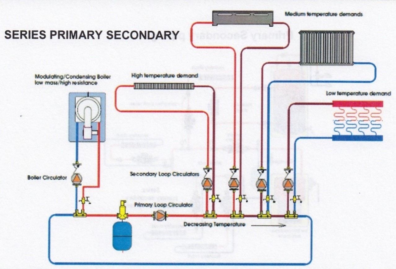
Once again, we see that 400 millinches per foot is the preferred range of friction loss for hydronic systems, as evidenced by the shaded column in the first table and the fact that the second table is based on 400 millinches per foot at various ΔTs. The sizes we would be most concerned with are for ½″ through 1½″, as these would be considered the pipe size and heat capacity range of most residential systems. In a primary/secondary system as seen in the graphic below, the boiler and primary loops would be sized according to the output of the boiler. Piping in any secondary loops would be sized according to the heat load of that particular loop.
Now complete the self-test questions.
Self-Test 2
Self-Test 2
- Which variety of PeX tubing is manufactured by the Engel method, and has a memory?
- PeX A
- PeX B
- PeX C
- PeX D
- Which variety of PeX tubing requires an oxygen-diffusion barrier when used in radiant floor panels?
- PeX A
- PeX B
- PeX C
- All of them
- What minimum thickness of rigid polystyrene foam should be placed under a basement concrete slab that is heated by radiant means?
- 1 inch
- 1 ½ inches
- 2 ½ inches
- 3 inches
- If a repair connection must be installed in a loop in a concrete-over-wood subfloor panel, where should the joint be located?
- In the ceiling below
- In the concrete first lift
- In the concrete second lift
- Somewhere above the concrete
- Which of the following is not a purpose of the wide, extra bottom plate in above-grade walls of a radiant floor panel system?
- To give the wall more stability
- To allow for carpet nailing strips
- To act as a screed for the second concrete lift
- To make up the 1 ½″ of ceiling height that the concrete takes from the room
- What would normally take place of a boiler in a snow melt system and effectively separates it from the building’s heating system, to prevent the entire system from having to be freeze protected?
- A pot feeder
- A water heater
- A heat exchanger
- A hydraulic separator
- What are radiant floor systems known as that heat the joist space below a floor?
- Wet systems
- Dry systems
- Air systems
- Hot systems
- What is installed along with batt insulation between joists that causes heat to be driven upward instead of downward?
- Reflective foil
- “Thermopan”
- Aluminum coils
- Absorption mats
- Which one of the following would be a false statement in regards to the installation of radiant ceiling panels?
- They operate at high temperatures
- They operate at low temperatures
- They don’t interfere with furniture placement
- They are out of reach of most people, for safety’s sake
- Which one of the following would be correct when laying radiant tubing loops in rooms that have one or two outside walls?
- Make a pass about 3 inches in along the outside walls and then right away go to a counterflow pattern
- Make two passes about 3 inches apart along the outside walls, then return back to the manifold
- Make a first pass about 6 inches from the outside walls, then turn 180° with another 6-inch pass, then resume normal loop layout
- Make two passes along the outside walls, then use a spiral loop layout for the rest of the room
- According to the tube centre spacing table, what is the suggested spacing for ½″ tubing if the floor output required were to be 27 BTUH/ft²?
- 12″ o.c.
- 9″ o.c.
- 6″ o.c.
- 4″ o.c.
- What is the maximum floor output from a radiant panel, in areas where people spend much time, over which supplemental heat will be necessary?
- 20 btuh/ft²
- 30 btuh/ft²
- 40 btuh/ft²
- 50 btuh/ft²
- What is generally the longest suggested loop length for ½″ radiant tubing at a 20°ΔT?
- 100 feet
- 300 feet
- 500 feet
- 1,000 feet
- What would be the tube spacing, floor output and total length of ½″ tube required in a kitchen if it had a gross area of 200 ft² and there were 42 ft² of lower wall cabinets, a range and fridge of 6.25 ft² each and an island of 30 ft²? The kitchen’s heat loss is estimated to be 3,050 btuh.
- Floor output = 21.75 btuh/ft²; tube spacing = 12″ o.c.; total length of tube = 115.5 ft
- Floor output = 18.30 btuh/ft²; tube spacing = 6″ o.c.; total length of tube = 150 ft
- Floor output = 12.91 btuh/ft²; tube spacing = 12″ o.c.; total length of tube = 200 ft
- Floor output = 26.41 btuh/ft²; tube spacing = 9″ o.c.; total length of tube = 150 ft
- What is normally used to locate tubing operating and embedded in a residential concrete floor?
- X-ray equipment
- An infra-red thermometer
- A metal detector
- A Polaroid camera
- Which multiplier would be used when determining the total tube required for a room with tubing laid at 6″ o.c. spacing?
- 1:1
- 1.3:1
- 2:1
- 3:1
- To what pressure, and for how long, should tubing be tested before being poured into a concrete mass?
- 100 psi for 10 minutes
- 100 psi for 30 minutes
- 50 psi for 10 minutes
- 50 psi for 30 minutes
- What main characteristic of a boiler is used when choosing it?
- Its input
- Its output
- Its fuel source
- Its efficiency
- When assigning a head loss to a circulator, what is used as the head loss for the piping?
- The single circuit with the highest head loss served by the pump
- The sum of all the head losses from all the circuits served by the pump
- The shortest measured single circuit served by the pump
- The sum of the two longest circuits served by the pump
- What are the two variables that are used in choosing a circulator?
- Psi and feet of head
- USGPM and flow rate
- Flow rate and feet of head
- Boiler output and size of piping
- From the pump graph shown below, without oversizing, pick the circulator that would deliver 140,000 BTUH at 12 feet of head.
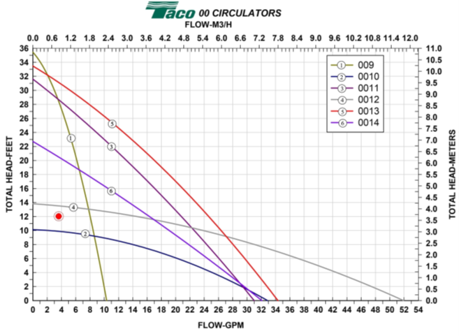
- #3
- #4
- #5
- #6
- What should the GPM flow rate be for a pump that is operating at a 5°FΔT and is supplying 48,000 BTUH?
- 19.2 GPM
- 9.6 GPM
- 6.4 GPM
- 4.8 GPM
- How many millinches are there in one foot?
- 12
- 64
- 1,000
- 12,000
- Using Table (A?) from the text, what is the head loss through 180 measured feet of pipe if friction losses are to be kept to within 400 millinches per foot?
- 4.5 feet
- 6 feet
- 7 feet
- 9 feet
- What variety of valve is a circuit setter?
- Gate
- Relief
- Globe
- Butterfly
- What is the name given to the strategy that uses a motorized mixing valve to automatically adjust its temperature setting in reaction to changing outdoor or system thermal conditions?
- Reset control
- Thermal mixing
- Thermostatic
- System monitor
- What is the term given to the practise of ensuring that the operation of one pump doesn’t affect the operation of another, if they share common piping?
- No-share strategy
- Hydraulic principle
- Hydraulic separation
- Point of no pressure change
- What characteristic of a brazed plate heat exchanger accounts for its high rate of heat transfer?
- Its number of ports
- Its inner plate surface area
- Its stainless-steel construction
- Its orientation (vertical vs horizontal)
- If a mixing valve has a CV of 3.2, what will be the pressure loss across it, in feet of head, if there needs to be enough flow to supply 37,000 btuh at a ΔT of 20°F?
- 1.35
- 1.60
- 3.09
- 3.70
- What type of valve can be installed between the supply and return mains that will open when the pressure in the supply main gets too high, as might happen when only one or two zone valves are open and there is only one system pump?
- An angle globe valve
- A backflow preventer
- A differential bypass valve
- An angle pressure relief valve
- If two pumps are installed in parallel with each other, the approximate will double.
- Flow rate
- Pressure
- Friction loss
- Temperature
- What should the proper air-side pressure be of a diaphragm-type expansion tank where the top of the system is 29 feet above the point of no pressure change and there is to be 5 psi at that point?
- 17.56 psi
- 15 psi
- 12.55 psi
- 5 psi
- Using the “Quick Method - Expansion Tank Sizing by Heat Capacity” and Table 2.5 Acceptance Volume and Table 2.6 Temp Conversion Factors, calculate the acceptance volume for a floor heating system using ½″ tubing that has a heat requirement of 45,000 BTUH and operates at 140°F if there is no glycol added?
- 1.00 USG
- 1.51 USG
- 2.02 USG
- 3.00 USG
- Which one of the following would not be a consideration of adding glycol to a heating system?
- Boiler operation
- Pump performance
- Expansion tank sizing
- Increased focus on backflow prevention
- According to Table 2.8 BTU Carrying Capacity of Pipe, in Thousands of BTU’s, based on 20°ΔT(temperature drop), what size would the boiler and primary loops be for a system whose boiler output was 65,000 BTUH?
- ¾″
- 1″
- 1 ¼″
- 1 ½″
Check your answers using the Self-Test Answer Keys in Appendix 1.
Media Attributions
- Figure 1 Tubing pattern for rooms with one outside wall by ITA is licensed under a CC BY-NC-SA licence.
- Figure 2 Tubing pattern for rooms with two outside walls by ITA is licensed under a CC BY-NC-SA licence.
- Figure 3 Tubing pattern for rooms with three outside walls by ITA is licensed under a CC BY-NC-SA licence.
- Figure 4 Tubing pattern for rooms with four or no outside walls (“counterflow”) by ITA is licensed under a CC BY-NC-SA licence.
- Figure 5 Radiant tubing layout patterns by ITA is licensed under a CC BY-NC-SA licence.
- Figure 6 Suggested loop fastening by ITA is licensed under a CC BY-NC-SA licence.
- Figure 7 Multiple Zone Valves with Single Circulator © Viega. Used with permission.
- Figure 8 Measuring circuit length is courtesy of TECA BC.
- Figure 9 Multiple Circulators for Zone Control © Viega. Used with permission.
- Figure 10 High head vs low head curves is courtesy of TECA BC.
- Figure 11 Circuit setter with PT plugs by ITA is licensed under a CC BY-NC-SA licence.
- Figure 12 3-way mixing valve © Viega. Used with permission.
- Figure 13 3-way valve in a primary-secondary system © Viega. Used with permission.
- Figure 14 4-way mixing valve © Viega. Used with permission.
- Figure 15 4-way mixing valve with radiant and high temperature DHW © Viega. Used with permission.
- Figure 16 Mixing valve actuator for modulating temperature control © Viega. Used with permission.
- Figure 17 Diverting valve © Viega. Used with permission.
- Figure 18 Diverting valve location © Viega. Used with permission.
- Figure 19 Mixing methods - injection mixing © Viega. Used with permission.
- Figure 20 Hydraulic separator © Viega. Used with permission.
- Figure 21 Hydraulic separation using closely-spaced tees © Viega. Used with permission.
- Figure 22 Brazed plate heat exchanger by ITA is licensed under a CC BY-NC-SA licence.
- Figure 23 Pump chart by ITA is licensed under a CC BY-NC-SA licence.
- Figure 24 Differential pressure valve by ITA is licensed under a CC BY-NC-SA licence.
- Figure 25 Multiple zones with single pump and DPV by ITA is licensed under a CC BY-NC-SA licence.
- Figure 26 Valved system using pressure-regulated ECM circulator © Viega. Used with permission.
- Figure 27 Two pumps in series will double the pressure, with unchanged flow rate © Viega. Used with permission.
- Figure 28 Two pumps in parallel will double the flow rate, with unchanged pressure © Viega. Used with permission.
- Figure 29 Diaphragm-style expansion tank cutaway by ITA is licensed under a CC BY-NC-SA licence.
- Figure 30 Primary/secondary system with secondary branch circuits © Viega. Used with permission.
