Appendix 3: Answers to Exercises
The following are suggested answers to the exercises embedded in the various chapters of Physical Geology. Answers to the chapter-end review questions are provided in Appendix 2.
Chapter 1
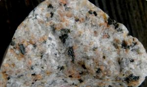
Exercise 1.1 Find a piece of granite
Responses will vary, but your sample should look something like the one shown below. Granitic rocks are hard and strong and difficult to break. They are dominated by feldspar (this one has both white plagioclase and pink potassium feldspar), but almost all have some quartz (which looks glassy) and a few dark minerals, like the black amphibole in this one.
Exercise 1.2 Plate motion during your lifetime
It depends where you live of course, but if you live anywhere in Canada and anywhere in the US east of the San Andreas fault, then you’re on the North America Plate, and that is moving towards the west at 2 to 2.5 cm/year. So if you’re around 20 years old, that plate has moved between 40 and 50 cm to the west in your lifetime.
Exercise 1.3 Using geological time notation
- 2.75 ka is 2,750 years.
- 0.93 Ga is 930,000,000 years or 930 million years.
- 14.2 Ma is 14,200,000 years or 14.2 million years.
Exercise 1.4 Take a trip through geological time
- The oxygenation of the atmosphere started at around 2.5 Ga (2500 Ma). It was a catastrophe for many organisms because they could not survive the strong oxidizing effects of free oxygen.
- We don’t really know the answer to this, but it’s not very long if you include insects, and there is evidence of insect damage to some of the earliest plants.
- Plants on land allowed for animals on land, so without land plants, we wouldn’t be here.
Chapter 2
Exercise 2.1 Cations, anions and ionic bonding
| Lithium (3) | Magnesium (12) | Argon (18) | Chlorine (17) | Beryllium (4) | Oxygen (8) | Sodium (11) |
|---|---|---|---|---|---|---|
| 2 in shell one and 1 in shell two | 2 in shell one, 8 in shell two and 2 in shell three | 2 in shell one, 8 in shell two and 8 in shell three | 2 in shell one, 8 in shell two and 7 in shell three | 2 in shell one and 2 in shell two | 2 in shell one and 6 in shell two | 2 in shell one, 8 in shell two and 1 in shell three |
| It loses an electron and becomes a +1 cation | It loses two electrons and becomes a +2 cation | It is electronically stable, and does not become an ion | It gains an electron and becomes a -1 anion | It loses two electrons and becomes a +2 cation | It gains two electrons and becomes a -2 anion | It loses an electron and becomes a +1 cation |
Exercise 2.2 Mineral groups
| Name | Formula | Group |
|---|---|---|
| sphalerite | ZnS | sulphide |
| magnetite | Fe3O4 | oxide |
| pyroxene | MgSiO3 | silicate |
| anglesite | PbSO4 | sulphate |
| sylvite | KCl | halide |
| silver | Ag | native |
| fluorite | CaF2 | halide |
| ilmenite | FeTiO3 | oxide |
| siderite | FeCO3 | carbonate |
| feldspar | KAlSi3O8 | silicate |
| sulphur | S | native |
| xenotime | YPO4 | phosphate |
Exercise 2.3 Make a tetrahedron
Responses will vary.
Exercise 2.4 Oxygen deprivation
Single chain silicate: 1:3 (silicon to oxygen). Double chain silicate: 7:19 (or 1:2.71)
Exercise 2.5 Ferromagnesian silicates
| Mineral | Formula | Ferromagnesian Silicate? |
|---|---|---|
| olivine | (Mg,Fe)2SiO4 | yes |
| pyrite | FeS2 | no (it’s a sulphide, not a silicate) |
| plagioclase | CaAl2Si2O8 | no |
| pyroxene | MgSiO3 | yes |
| hematite | Fe2O3 | no (it’s an oxide, not a silicate) |
| orthoclase | KAlSi3O8 | no |
| quartz | SiO2 | no |
| amphibole | Fe7Si8O22(OH)2 | yes |
| muscovite | K2Al4 Si6Al2O20(OH)4 | no |
| magnetite | Fe3O4 | no (it’s an oxide, not a silicate) |
| biotite | K2Fe4Al2Si6Al4O20(OH)4 | yes |
| dolomite | (Ca,Mg)CO3 | no (it’s a carbonate, not a silicate) |
| garnet | Fe2Al2Si3O12 | yes |
| serpentine | Mg3Si2O5(OH)4 | yes |
Chapter 3
Exercise 3.1 Rock around the rock-cycle clock
Sedimentary rock is buried deeper to make metamorphic rock, the metamorphic rock is uplifted and during this process the material overhead is eroded so that it can be exposed at surface. The metamorphic rock is then eroded to make more sediments, which are deposited and then buried to make sedimentary rock. This would likely take at least 60 million years.
Exercise 3.2 Making magma viscous
Responses will vary.
Exercise 3.3 Rock types based on magma composition
| Rock Sample | SiO2 | Al2O3 | FeO | CaO | MgO | Na2O | K2O | What type of magma is it? |
|---|---|---|---|---|---|---|---|---|
| Rock 1 | 55% | 17% | 5% | 6% | 3% | 4% | 3% | intermediate (although the SiO2 level is borderline, there is too little FeO, MgO and CaO to be mafic) |
| Rock 2 | 74% | 14% | 3% | 3% | 0.5% | 5% | 4% | felsic |
| Rock 3 | 47% | 14% | 8% | 10% | 8% | 1% | 2% | mafic |
| Rock 4 | 65% | 14% | 4% | 5% | 4% | 3% | 3% | intermediate (although the SiO2 level is borderline, there is too much MgO and CaO to be felsic) |
Exercise 3.4 Porphyritic minerals
- only olivine phenocrysts
- pyroxene and amphibole phenocrysts, along with plagioclase with a composition that is about half-way between the Ca-rich and the Na-rich end-members.
Exercise 3.5 Mineral proportions in igneous rocks
- Roughly 25% K-feldspar, 30% quartz, 35% albitic plagioclase and 10 biotite/amphibole,
- Roughly 65% plagioclase and 35% biotite/amphibole (most likely amphibole),
- Roughly 45% anorthitic plagioclase, 25% amphibole and 35% pyroxene
- Roughly 50% pyroxene and 50% olivine.
Exercise 3.6 Proportions of Ferromagnesian Silicates
The approximate proportions are: 10%, 50%, 30% and 2%, and the corresponding rock names are granite, gabbro (although it’s right on the boundary between gabbro and diorite), diorite and granite.
Exercise 3.7 Pluton Problems
- a stock
- a dyke (it cuts across bedding and the granite)
- a sill (it is parallel to bedding)
- a dyke
- a sill
Chapter 4
Exercise 4.1 How thick is the oceanic crust?
The magma available to create oceanic crust at this setting is approximately 10% of the volume of the 60 kilometres thick part of the mantle from which it is derived, so the oceanic crust should be about 6 kilometres thick.
Exercise 4.2 Under pressure
No answer possible.
Exercise 4.3 Volcanoes and subduction
The volcanoes are between 200 and 300 kilometres from the subduction boundary, about 250 kilometres on average. If the subducting crust is descending at 40 kilometres per 100 kilometres inland, the depth to the Juan de Plate beneath these volcanoes is between 80 and 120 kilometres , or 100 kilometres on average.
Exercise 4.4 Kilauea’s June 27th lava flow
- The flow front advanced at a rate of about 160 metres per day or just under 7 metres per hour between June 27th and October 29th 2014. That doesn’t mean that the lava only flowed at rates of a few metres per hour over that time. It likely flowed much faster (probably 10s to 100s of metres per hour), but it advanced in fits and starts, and the advancing front changed locations many times. At other times the flow spread out across the area.
- Between January 2015 and January 2016 the flow did not extend any further northeast towards Pahoa. Instead it spread out across the plain to the north of Pu’ u’ o’ o.
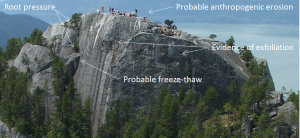
Exercise 4.5 Volcanic hazards in Squamish
| Hazard | Risk |
|---|---|
| 1. Tephra emission | Yes. However, much of the tephra from a large eruption would extend up into the atmosphere, and would not affect Squamish. |
| 2. Gas emission | Yes. There could be dangerous amounts of sulphurous or acidic gases flowing down the mountainside into Squamish. |
| 3. Pyroclastic density current | Yes. A pyroclastic density current that flows down the western or southwestern sides of Garibaldi could easily reach Squamish. |
| 4. Pyroclastic fall | Yes. In the later stages of a large eruption some tephra (or pyroclastic fragments) could rain down on Squamish |
| 5. Lahar | Yes. Squamish is definitely at risk from a lahar on the western side of the mountain. The risk would be increased if the eruption takes place in winter or spring when the amount of snow is at a maximum. |
| 6. Sector collapse | Yes, this is possible. The western side of Mt. Garibaldi has already collapsed several times since the last glaciation. |
| 7. Lava flow | Yes. Squamish is at risk from lava that flows on the southern and western sides of the mountain. There is a Pleistocene-aged lava flow clearly evident in the photograph. It flowed down the southern flank, and then turned west towards where Squamish is situated today. |
Exercise 4.6 Volcano alert!
The most important tools for monitoring volcanoes are seismometers, and while there is a good network of seismometers in southwestern BC, there are not enough in close proximity to Mount Garibaldi to be able to accurately define the locations and depths of earthquakes around the volcano. So the first project would be to establish about 5 additional seismic stations in the Squamish region. They don’t have to be right on the mountain, but can be placed near to existing roads and highways in the area. They need to be secured to bedrock. Every effort should be made to have them located on all sides of the mountain. The second project would be to establish some means of measuring deformation of the mountain itself. This could be done with tiltmeters or GPS stations, but GPS would be better. The GPS receivers have to be placed on the flanks of the mountain, and they also have to be installed right on bedrock. That could be a real challenge in winter or spring, when there is lots of snow. While this work is going on, we should charter a helicopter to fly around the mountain to see if there is any sign of eruptive activity or melting snow, and to look for convenient places to install GPS stations. We may want to land in a few different places.
There isn’t a lot that we can say to the public at this stage, except that this sudden increase in seismic activity could mean that Garibaldi is getting ready to erupt, that the Geological Survey and all emergency measures organizations are working together on it, and that residents of the Squamish area, and anyone using highway 99, should keep listening to local radio stations for further updates. We could also establish a system to send out alerts via text message.
Exercise 4.7 Volcanoes down under
We would expect to see composite volcanoes on the North Island, some 200 to 300 kilometres inland (northwest) from the Kermadec Trench, and within the ocean along the same trend to the northeast of New Zeland. There is also the potential for composite volcanism to the south of the South Island, east of the Macquarrie fault zone, although there appears to be some doubt about whether subduction is actually taking place in this region.
Chapter 5
Exercise 5.1 Mechanical weathering
Exercise 5.2 Chemical weathering
| Chemical change | Process |
|---|---|
| 1. Pyrite to hematite | oxidation |
| 2. Calcite to calcium and bicarbonate ions | dissolution |
| 3. Feldspar to clay | hydrolysis |
| 4. Olivine to serpentine | hydrolysis |
| 5. Pyroxene to iron oxide | oxidation |
Exercise 5.3 Describing the weathering origins of sands
| Sand description | Possible processes |
|---|---|
| Fragments of coral etc. from a shallow water area near to a reef in Belize | Reefs are constantly being eroded by ocean waves, and the fragments are washed inshore by currents and then further eroded by wave action. |
| Angular quartz and rock fragments from a glacial stream deposit near Osoyoos | Quartz-bearing rocks have been eroded and transported by a glacier. The fragments may have been moved a short distance by a stream, but not enough to produce rounding. |
| Rounded grains of olivine and volcanic glass from a beach in Hawaii | The olivine and glass grains are eroded by waves from volcanic rock and then thoroughly rounded by waves on the beach |
Exercise 5.4 The soils of Canada
| Soil type | Distribution | Explanation |
|---|---|---|
| 1. Chernozem | Southern prairies | These are dry-climate soils developed on grasslands |
| 2. Luvisol | Northern prairies and BC interior | Soils developed on sedimentary rocks in cool moist climates |
| 3. Podsol | Mountainous parts of BC and large parts of northern Ontario and Quebec | Areas with coniferous forests and moderate climates |
| 4. Brunisol | Boreal forest regions | Cold forested regions with discontinuous permafrost |
| 5. Organic | Hudson Bay and James Bay lowlands | Wetland areas with widespread swamps |
Chapter 6
Exercise 6.1 Describe the sediment on a beach
Responses will vary.
Exercise 6.2 Classifying sandstones
| Description | Rock name |
|---|---|
| Angular grains, 85% quartz, 15% feldspar, less than 5% silt and clay | Arkosic arenite |
| Rounded grains, 99% quartz, less than 2% silt and clay | Quartz arenite |
| Angular grains, 70% quartz, 20% lithic and 10% feldspar, roughly 20% silt and clay | Lithic wacke |
Exercise 6.3 Making evaporite
Responses will vary.
Exercise 6.4 Interpretation of past environments
| Description | Source rock | Weathering | Transportation | Dep. environment |
|---|---|---|---|---|
| 1. Cross-bedded quartz sandstone, rounded grains | probably sandstone | strong chemical weathering | wind | desert |
| 2. Feldspathic sandstone and mudstone with volcanic fragments and repetitive graded bedding | granite and volcanic rock | weak chemical weathering | short transport in a river | sub-marine fan |
| 3. Conglomerate with well- rounded pebbles and cobbles, imbricated | granite and volcanic rock | difficult to tell | high-energy river | moderate energy river |
| 4. Limestone breccia with orange-red matrix | limestone | mechanical only | rock fall | talus slope, oxidizing environment |
Chapter 7
Exercise 7.1 How long did it take?
It might have taken in the order of 20 to 25 million years for these garnets to form, but even more time is needed than that to produce the rock because we have to account for the sedimentary process and then burial and lithification and then deeper burial to reach metamorphic environment – several tens of millions more years.
Exercise 7.2 Naming metamorphic rocks
| Rock Description | Name |
|---|---|
| 1. A rock with visible minerals of mica and with small crystals of andalusite. The mica crystals are consistently parallel to one another. | Schist or (preferably) Mica-andalusite schist |
| 2. A very hard rock with a granular appearance and a glassy lustre. There is no evidence of foliation. | Probably quartzite |
| 3. A fine-grained rock that splits into wavy sheets. The surfaces of the sheets have a sheen to them. | Phyllite |
| 4. A rock that is dominated by aligned crystals of amphibole. | Amphibolite |
Exercise 7.3 Metamorphic rocks in areas with higher geothermal gradients
| Metamorphic Rock Type | Depth (km) |
|---|---|
| 1. Slate | 2 to 5 |
| 2. Phyllite | 5 to 8 |
| 3. Schist | 8 to 12 |
| 4. Gneiss | 12 to 17 |
| 5. Migmatite | 17 to 25 |
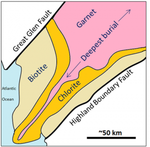
Exercise 7.4 Scottish metamorphic zones
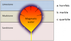
Exercise 7.5 Contact metamorphism and metasomatism
Review: Rock or Mineral?
| Mineral or Rock Name | Rock or Mineral? | If it’s a mineral, which group does it belong to? If it’s a rock, what type is it? |
|---|---|---|
| Feldspar | Mineral | Silicate |
| Calcite | Mineral | Carbonate |
| Slate | Rock | Metamorphic (regional) |
| Hematite | Mineral | Oxide |
| Rhyolite | Rock | Volcanic igneous |
| Sandstone | Rock | Clastic sedimentary |
| Diorite | Rock | Intrusive igneous |
| Olivine | Mineral | Silicate |
| Pyrite | Mineral | Sulphide |
| Quartzite | Rock | Metamorphic (regional or contact) |
| Granite | Rock | Intrusive igneous |
| Amphibole | Mineral | Silicate |
| Conglomerate | Rock | Clastic sedimentary |
| Chert | Rock | Chemical sedimentary |
| Halite | Mineral | Halide |
| Gneiss | Rock | Metamorphic (regional) |
| Mica | Mineral | Silicate |
| Pyroxene | Mineral | Silicate |
| Chlorite | Mineral | Silicate |
| Limestone | Rock | Chemical sedimentary |
| Andesite | Rock | Volcanic igneous |
Chapter 8
Exercise 8.1 Cross-cutting relationships
![Relative ages: 2: oldest: 3: middle, 1: youngest [SE]](https://opentextbc.ca/physicalgeology2ed/wp-content/uploads/sites/298/2019/08/ex8-1-300x269-1.png)
Exercise 8.2 Dating rocks using index fossils
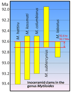
The age of the rock is probably between 92.6 and 92.7 Ma. If M. subhercynius was not present, the age range would be between 92.6 and 92.9 Ma
Exercise 8.3 Isotopic dating
![Isotopic dating [SE]](https://opentextbc.ca/physicalgeology2ed/wp-content/uploads/sites/298/2019/08/ex8-3-300x182-1.png)
With a ratio of 0.91 the age is 175 Ma (red dotted line).
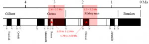
Exercise 8.4 Magnetic dating
The possible age ranges are 3.05 to 3.12 Ma and 1.78 to 2.00 Ma
Exercise 8.5 What happened on your birthday?
Answers will vary.
Chapter 9
Exercise 9.1 How soon will seismic waves get here?
Times shown for velocity of 5 kilometres per second (km/s).
- Nanaimo (120 kilometres), 24 seconds.
- Surrey (200 kilometres), 40 seconds.
- Kamloops (390 kilometres), 78 seconds.
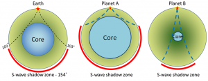
Exercise 9.2 Liquid cores in other planets
Exercise 9.3 What does your magnetic dip meter tell you?
- Up at a shallow angle: Southern hemisphere, near the equator.
- Parallel to the ground: Equator.
- Down at a steep angle: Northern hemisphere, near the pole.
- Straight down: North pole.
Exercise 9.4 Rock density and isostasy
| Rock Type | Volumes of individual minerals in 1000 cm3 | Grams of individual minerals in 1000 cm3 | Total Weight (grams) | Density (grams per cubic centimetre, g/cm3) |
|---|---|---|---|---|
| Continental Crust (Granite) | Quartz - 180 cm3
Feldspar - 760 cm3 Amphibole - 70 cm3 |
Quartz - 477 g
Feldspar - 1999 g Amphibole - 277 g |
2703 g | 2.70 |
| Oceanic Crust (Basalt) | Feldspar - 450 cm3
Amphibole - 50 cm3 Pyroxene - 500 cm3 |
Feldspar - 1184 g
Amphibole - 164 g Pyroxene - 1700 g |
3048 g | 3.05 |
| Mantle (Peridotite) | Pyroxene - 450 cm3
Olivine - 550 cm3 |
Pyroxene - 1530 g
Olivine - 1815 g |
3345 g | 3.35 |
Chapter 10
Exercise 10.1 Fitting the continents together
![Pangea [SE]](https://opentextbc.ca/physicalgeology2ed/wp-content/uploads/sites/298/2019/08/ex10-1-227x300-1.png)
Exercise 10.2 Volcanoes and the rate of plate motion
![Pacific Plate rates of motion [SE]](https://opentextbc.ca/physicalgeology2ed/wp-content/uploads/sites/298/2019/08/ex10-2-274x300-1.png)
Exercise 10.3 Paper transform fault model
No answer possible.
Exercise 10.4 A different type of transform fault
![Juan de Fuca and Explorer Plates [SE]](https://opentextbc.ca/physicalgeology2ed/wp-content/uploads/sites/298/2019/08/ex10-4-280x300-1.png)
The Juan de Fuca Plate is moving faster than the Explorer Plate, which means that the Juan de Fuca Plate is sliding past the Explorer Plate. There is side-by-side relative motion on this plate boundary, and that makes it a transform fault.
Exercise 10.5 Getting to know the plates and their boundaries
![The extents of the Earth's major plates [SE]](https://opentextbc.ca/physicalgeology2ed/wp-content/uploads/sites/298/2019/08/ex10-5-300x170-1.png)
Chapter 11
Exercise 11.1 Earthquakes in British Columbia
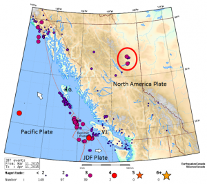
- Most of the earthquakes between the Juan de Fuca (JDF) and Explorer Plates are related to transform motion along that plate boundary,
- The string of small earthquakes adjacent to Haida Gwaii are likely aftershocks of the 2012 M7.7 earthquake in that area.
- Most of the earthquakes around Vancouver Island (V.I.) are related to deformation of the North America Plate continental crust by compression along the subduction zone.
- Earthquakes that are probably caused by fracking are enclosed within a red circle on the map.
Exercise 11.2 Moment magnitude estimates from earthquake Parameters
| Length (km) | Width (km) | Displacement (m) | Comments | MW? |
|---|---|---|---|---|
| 60 | 15 | 4 | The 1946 Vancouver Island earthquake | 7.3 |
| 0.4 | 0.2 | .5 | The small Vancouver Island earthquake shown in Figure 11.13 | 4.0 |
| 20 | 8 | 4 | The 2001 Nisqually earthquake described in Exercise 11.3 | 6.8 |
| 1,100 | 120 | 10 | The 2004 Indian Ocean earthquake | 9.0 |
| 30 | 11 | 4 | The 2010 Haiti earthquake | 7.0 |
The largest recorded earthquake had a magnitude of 9.5. Could there be a 10?
To have a magnitude of 10, one possible solution is 2500 kilometres long and 300 kilometres wide with 55 metres of displacement. (Other solutions are possible.) These are unreasonable numbers because subduction zones don’t tend to fail over that length (typically not much more than 1200 kilometres), rupture zones cannot be that wide because that takes us into the asthenosphere, and displacements are never likely to be that great.
Exercise 11.3 Estimating intensity from personal observations
| Building Type | Floor | Shaking Felt | Lasted (seconds) | Description of Motion | Intensity? |
|---|---|---|---|---|---|
| House | 1 | no | 10 | Heard a large rumble lasting not even 10 s, mirror swayed | 2 |
| House | 2 | moderate | 60 | Candles, pictures & CDs on bookshelf moved, towels fell off racks | 4 |
| House | 1 | no | Pots hanging over stove moved and crashed together | 3 | |
| House | 1 | weak | Rolling feeling with a sudden stop, picture fell off mantle, chair moved | 4 | |
| Apartment | 1 | weak | 10 | Sounded like a big truck then everything shook for a short period | 3 |
| House | 1 | moderate | 20-30 | Teacups rattled but didn't fall off | 3 |
| Institution | 2 | moderate | 15 | Creaking sounds, swaying movement of shelving | 3 |
| House | 1 | moderate | 15-30 | Bed banging against the wall with me in it, dog barking aggressively | 4 |
Exercise 11.4 Creating liquefaction and discovering the harmonic frequency
No answer possible.
Exercise 11.5 Is your local school on the seismic upgrade list?
Answers will vary.
Chapter 12
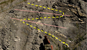
Exercise 12.1 Folding style
In order to help with the interpretation, one of the beds has been traced (in yellow) on the diagram below, and two of the fold axes have been shown (in pink). These folds are symmetrical, and although they are tight they are not isoclinal. They are overturned.
Exercise 12.2 Types of faults
| Top left: a normal fault, implying extension |
| Bottom left: a series of normal faults, extension |
| Top right: A reverse fault, compression |
| Bottom right: a right lateral fault (implies that there is shearing, but it is not possible to say if there is extension or compression) |
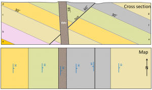
Exercise 12.3 Putting strike and dip on a map here!
See map below for strike and dip symbols. Relative ages, from youngest to oldest:
- dyke (youngest)
- fault
- layer g (although this layer isn’t intersected by the fault or the dyke so it is not possible to know that it is older based on the information available)
- layer f
- layer e
- layer d
- layer c
- layer b
- layer a (oldest)
Chapter 13
Exercise 13.1 How long does water stay in the atmosphere?
The volume of the oceans is 1,338,000,000 km3 and the flux rate is approximately the same (1,580 km3/day).
What is the average residence time of a water molecule in the ocean?
1,338,000,000/1,580 = 846,835 days average residence time for water in the ocean (or 2320 years)
Exercise 13.2 The effect of a dam on base level
How does the formation of a reservoir affect the stream where it enters the reservoir, and what happens to the sediment it was carrying?
The velocity of the streams slows to zero and most of the sediment is deposited quickly.
The water leaving the dam has no sediment in it. How does this affect the stream below the dam?
With nothing to deposit, the water below the dam can only erode, so there will be enhanced erosion below the dam.
Exercise 13.3 Understanding the Hjulström-Sundborg Diagram
![[SE]](https://opentextbc.ca/physicalgeology2ed/wp-content/uploads/sites/298/2019/08/ex13-3-300x205-1.png)
- A fine sand grain (0.1 millimetres) is resting on the bottom of a stream bed.
- What stream velocity will it take to get that sand grain into suspension? Roughly 20 centimetres per second.
- Once the particle is in suspension, the velocity starts to drop. At what velocity will it finally come back to rest on the stream bed? Roughly 1 centimetres per second.
- A stream is flowing at 10 centimetres per second (which means it takes 10 seconds to go 1 metre, and that’s pretty slow).
- What size of particles can be eroded at 10 centimetres per second? No particles, of any size, will be eroded at 10 centimetres per second, although particles smaller than 1 millimetre that are already in suspension will stay in suspension.
- What is the largest particle that, once already in suspension, will remain in suspension at 10 centimetres per second? A 1 millimetre diameter particle should remain in suspension at 10 centimetres per second.
Exercise 13.4 Determining stream gradients
![Gradients of Priest Creek [SE]](https://opentextbc.ca/physicalgeology2ed/wp-content/uploads/sites/298/2019/08/ex13-4-300x300-1.png)
The length of the creek between 1,600 metres and 1,300 metres elevation is 2.4 kilometres, so the gradient is 300 divided by 2.4 = 125 metres per kilometre.
- Use the scale bar to estimate the distance between 1,300 metres and 600 metres and then calculate that gradient. 5.2 kilometres, with a gradient of 700 divided by 5.2 = 134 metres per kilometre.
- Estimate the gradient between 600 metres and 400 metres. 3.6 kilometres, with a gradient of 200 divided by 3.6 = 56 metres per kilometre.
- Estimate the gradient between 400 metres on Priest Creek and the point where Mission Creek enters Okanagan Lake. 4 kilometres, with a gradient of 60 divided by 4.0 = 15 metres per kilometre.
Exercise 13.5 Flood probability on the Bow River
- Calculate the recurrence interval for the second largest flood (1932, 1,520 m3/s). Ri = 96/2 = 48 years
- What is the probability that a flood of 1,520 m3/s will happen next year? 1/48 = 0.02 or 2%
- Examine the 100-year trend for floods on the Bow River. If you ignore the major floods (the labelled ones), what is the general trend of peak discharges over that time? In general the peak discharges are getting lower (from an average of around 400 m3/s in 1915 to an average of about 300 m3/s in 2015)
Chapter 14
Exercise 14.1 How long will it take?
[latex]i=\dfrac{37\text{ m}-21\text{ m}}{80\text{ m}}=0.2, K=0.0002 \text{ m/s},[/latex] and [latex]n=0.25,[/latex] so [latex]V=\dfrac{0.0002\text{ m/s}\times 0.2}{0.25}=0.00016\text{ m/s}.[/latex]
At that rate, it will take 500,000 seconds for the groundwater to flow from the gas station to the stream. That converts to 138 hours, or about 6 days.
Exercise 14.2 Cone of depression
The cone of depression increases the gradient of the water table in the area around the well. That should increase the rate at which water flows towards the well.
Exercise 14.3 What is your water table doing?
![[BC Ministry of the Environment at http://www.env.gov.bc.ca/wsd/data_searches/obswell/map/]](https://opentextbc.ca/physicalgeology2ed/wp-content/uploads/sites/298/2019/08/ex14-3-300x251-1.png)
The water-level for a random observation well in BC is shown above. The water table is slowly rising at this location. Since 2004 the lowest water level has risen from just above 4 m below surface to around 3.6 m above surface and the highest level has risen from around 0.3 m below surface to nearly at surface (0 m). Prior to 2004, where the points are not joined with lines, the trend appears to be similar.
Exercise 14.4 What goes on at your landfill?
Responses will vary.
Exercise 14.5 Finding a leaking UST in your community
Responses will vary.
Exercise 14.6 Manipulating a contaminant plume
What could you do at wells A and C to prevent this? Explain and use the diagram below to illustrate the expected changes to the water table and the movement of the plume.
![Implications of pumping from wells B and C and injecting into well A [SE]](https://opentextbc.ca/physicalgeology2ed/wp-content/uploads/sites/298/2019/08/ex14-6-300x129.png)
Possible Answer: Injection into well A will cause water table to rise there (like the reverse of a cone of depression), thus reversing flow direction to the right of well A and moving the plume towards Well B. Extraction from Wells B and C will cause cones of depression and help to reverse the flow and pull the plume back from the stream. Both wells B and C may receive contaminants and so the water from both may need treatment.
Chapter 15
Exercise 15.1 Sand and water
Responses will vary.
Exercise 15.2 Classifying slope failures
![[SE]](https://opentextbc.ca/physicalgeology2ed/wp-content/uploads/sites/298/2019/08/ex15-2-300x261.png)
Exercise 15.3 How much does a house weigh and can it contribute to a slope failure?
A typical 150 m2 (approximately 1,600 ft2) wood-frame house with a basement and a concrete foundation weighs about 145 t (metric tonnes). But most houses are built on foundations that are excavated into the ground. This involves digging a hole and taking some material away, so we need to subtract what that excavated material weighs. Assuming our 150 m2 house required an excavation that was 15 m by 11 m by 1 m deep, that’s 165 m3 of “dirt,” which typically has a density of about 1.6 t per m3.
165 m3 of excavated soil × 1.6 t/m3 = 264 t – thus the excavated material weighs about 1.8 times as much as the house. In this case weight has been removed from the slope by building the house.
Chapter 16
Exercise 16.1 Pleistocene glacials and interglacials
Describe the nature of temperature change that followed each of these glacial periods.
In each case the temperature drops slowly building to a peak of glaciation, and then each of the glacial periods is followed by a very rapid increase in temperature.
The current interglacial (Holocene) is marked with an H. Point out the previous five interglacial periods.
The previous 5 interglacials are labelled 1 to 5 on the diagram below. Interglacial 2 had two distinct warm episodes.
![[SE]](https://opentextbc.ca/physicalgeology2ed/wp-content/uploads/sites/298/2019/08/ex16-1-300x178.png)
Exercise 16.2 Ice advance and retreat
![Glacial advance (top) and retreat (bottom) [SE]](https://opentextbc.ca/physicalgeology2ed/wp-content/uploads/sites/298/2019/08/ex16-2-300x150.png)
The red dots show the new positions of the markers.
Exercise 16.3 Identify glacial erosion features
- col
- arête
- horn
- cirque
- truncated spur (other arêtes are labelled in the image)
![[SE after http://en.wikipedia.org/wiki/Mount_Assiniboine#/media/File:Mount_Assiniboine_Sunburst_Lake.jpg]](https://opentextbc.ca/physicalgeology2ed/wp-content/uploads/sites/298/2019/08/ex16-3-300x185.png)
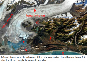
Exercise 16.4 Identify glacial depositional environments
Chapter 17
Exercise 17.1 Wave height versus length
This table shows the typical amplitudes and wavelengths of waves generated under different wind conditions. The steepness of a wave can be determined from these numbers and is related to the ratio: amplitude/wavelength.
- Calculate these ratios for the waves shown.
- How would these ratios change with increasing distance from the wind that produced the waves?
| Amplitude (metres) | Wavelength (metres) | Ratio (amplitude/wavelength) |
|---|---|---|
| 0.27 | 8.5 | 0.03 |
| 1.5 | 33.8 | 0.04 |
| 4.1 | 76.5 | 0.05 |
| 8.5 | 136 | 0.06 |
| 14.8 | 212 | 0.07 |
Within increasing distance from the source the wave heights would gradually decrease and so the ratios would decrease.
Exercise 17.2 Wave refraction
![[SE]](https://opentextbc.ca/physicalgeology2ed/wp-content/uploads/sites/298/2019/08/ex17-2-300x144.png)
Exercise 17.3 Beach forms
Barrier islands could from if this was a low-relief coast with an abundant supply of sediment from large rivers.
![Possible locations of coastal deposits [SE]](https://opentextbc.ca/physicalgeology2ed/wp-content/uploads/sites/298/2019/08/ex17-3-300x201.png)
Exercise 17.4 A Holocene uplifted shore
The melting of glacial ice around the world at the end of the last glaciation (between 14 and 8 ka – see Figure 17.25) led to relatively rapid sea-level rise (by a total of approximately 125 m) which resulted in this area being submerged. That was a eustatic process. In response to the loss of ice in this region of coastal British Columbia there was a slower isostatic rebound of the crust, which is why this area is now back up above sea level.
Exercise 17.5 Crescent Beach groynes
![[SE]](https://opentextbc.ca/physicalgeology2ed/wp-content/uploads/sites/298/2019/08/ex17-5-300x124.png)
Chapter 18
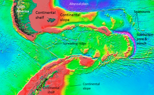
Exercise 18.1 Visualizing sea-floor topography
- see map, below
- This is the area between the southern tip of South America (Cape Horn) and the Antarctic Peninsula. The body of water between the two is the Drake Passage.
Exercise 18.2 The age of subducting crust
- The oldest is in the southeast and is greater than 8 Ma (see map below).
- The youngest is in the north and is close to 0 Ma.
![[SE]](https://opentextbc.ca/physicalgeology2ed/wp-content/uploads/sites/298/2019/08/ex18-2-228x300.png)
Exercise 18.3 What type of sediment
-
- siliceous ooze or clay
- carbonate ooze
- siliceous ooze or clay
- coarse terrigenous or carbonate ooze
![[SE]](https://opentextbc.ca/physicalgeology2ed/wp-content/uploads/sites/298/2019/08/ex18-3-300x96.png)
Exercise 18.4 Salt chuck
No answer possible.
Exercise 18.5 Understanding the Coriolis effect
No answer possible.
Chapter 19
Exercise 19.1 Climate Change at the K-Pg Boundary
The short-term climate impact was significant cooling because the dust (and sulphate aerosols) would have blocked incoming sunlight. This effect may have lasted for several years, but its intensity would have decreased over time.
The longer-term impact would have been warming caused by the greenhouse effect of the carbon dioxide.
Exercise 19.2 Albedo Implications of Forest Harvesting
Clear-cutting (or any logging activity) leads to a net increase in albedo, so the albedo-only impact is cooling.
Exercise 19.3 What Does Radiative Forcing Tell Us?
Using the ΔT = ΔF * 0.8 equation the expected temperatures for 2011, 1980 and 1950 compared with the estimated 13.4 C in 1750 should be:
2011 vs 1750 ΔT = 0.8 * 2.29 = 1.8°C (13.4 + 1.8 = 15.2)
1980 vs 1750 ΔT = 0.8 * 1.25 = 1.0°C (13.4 + 1.0 = 14.4)
1950 vs 1750 ΔT = 0.8 * 0.57 = 0.5°C (13.4 + 0.5 = 13.9)
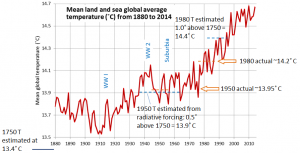
Based on this reasoning the estimated temperature for 1950 is13.9˚ C (which is close to the actual of 14.0 ˚ C), while that for 1980 is 14.4˚ C, which is well above the actual of 14.2˚ C. It’s also clear that we didn’t reach 15.2˚ C by 2011, because even in the hottest year so far (2015) the global average temperature was only 14.8˚ C.
So while the ΔT = ΔF * 0.8 equation is useful, it appears to overestimate the temperature, probably because it takes some time (years to decades) for the climate to catch up to the forcing.
Exercise 19.4 Rainfall and ENSO
Describe the relationship between ENSO and precipitation in B.C.’s southern interior.
As shown on the diagram below, there are some examples where a strong ENSO signal corresponds with very strong precipitation in the interior (and on the coast as well). The two strongest El Niños (1983 and 1998) shown correspond with the highest recorded precipitation levels in Penticton. Some other strong El Niños (1958 and 1973) are associated with strong precipitation within 6 months of the ENSO peak, but others show a negative correlation between ENSO and rainfall (marked with “?”).
![[SE using climate data from Environment Canada, and ENSO data from: http://www.esrl.noaa.gov/psd/enso/mei/table.html]](https://opentextbc.ca/physicalgeology2ed/wp-content/uploads/sites/298/2019/08/ex19-4-300x153.png)
Exercise 19.5 How Can You Reduce Your Impact on the Climate?
Responses will vary.
Chapter 20
Exercise 20.1 Where does it come from?
Responses will vary.
Exercise 20.2 The importance of heat and heat engines
| Deposit Type | Is Heat a Factor? | If So, What Is the Role of the Heat? |
|---|---|---|
| Magmatic | Yes | Heat is necessary for melting of the rock to produce magma |
| Volcanogenic massive sulphide | Yes | Heat is necessary for melting of the rock to produce magma |
| Porphyry | Yes | Heat contained within the porphyritic intrusion drives the convection system |
| Banded iron formation | No | Iron is deposited from cold ocean water |
| Unconformity-type uranium | Probably | Uranium solubility is enhanced at higher water temperatures |
Exercise 20.3 Sources of important lighter metals
| Element | Silicon | Calcium | Sodium | Potassium | Magnesium |
|---|---|---|---|---|---|
| Source(s) | quartz sand | lime-stone | halite (NaCl) | sylvite (KCl) | dolomite ((Ca,Mg)CO3), magnesite (MgCO3), salt lakes and the ocean |
Exercise 20.4 Interpreting a seismic profile
![[SE after USGS at: http://walrus.wr.usgs.gov/infobank/programs/html/definition/seis.html]](https://opentextbc.ca/physicalgeology2ed/wp-content/uploads/sites/298/2019/08/ex20-4-300x167.png)
Chapter 21
Exercise 21.1 Finding the Geological Provinces of Canada
![[SE after Geological Survey of Canada]](https://opentextbc.ca/physicalgeology2ed/wp-content/uploads/sites/298/2019/08/ex21-1-300x233.png)
Exercise 21.2 Purcell Rocks Down Under?
The Mesoproterozoic quartzite phyllite schist of Tasmania may correlate with the Purcell rocks of Canada. The main difference is that while the Tasmanian rocks are metamorphosed, the Purcell rocks are generally unmetamorphosed.
Exercise 21.3 What Is Vancouver Island Made Of?
- Less than 10% of Vancouver Island is Paleozoic (the Devonian volcanic rocks - Dv).
- The most common rock type is the Triassic Karmutsen Volcanic rock (basalt - Tv). The most common rocks by age are the Mesozoic rocks (Jurassic volcanic, Jurassic granite and Triassic volcanic).
![[SE]](https://opentextbc.ca/physicalgeology2ed/wp-content/uploads/sites/298/2019/08/ex21-3-300x229.png)
Exercise 21.4 Dinosaur country?
This Cretaceous Dinosaur Park Formation sandstone is clearly cross-bedded implying that it was deposited in a stream environment.
Exercise 21.5 The volume of the Paskapoo Formation
- The 60,000 km2 area of source rock would have to have been eroded to a depth of 750 m to create 45,000 km3 of sediment
- 500 m is 500,000 mm so the rate is 500,000 mm/ 4,000,000 years = 0.125 mm/year
Chapter 22
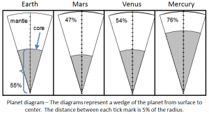
Exercise 22.1 How do we know what other planets are like inside?
| Description | Earth | Mars | Venus | Mercury |
|---|---|---|---|---|
| Planet density (uncompressed) in g/cm3 | 4.05 | 3.74 | 4.00 | 5.30 |
| Percent core | 16.8% | 10.3% | 15.8% | 43.2% |
| Description | Earth | Mars | Venus | Mercury |
|---|---|---|---|---|
| Unsqueezed planet volume - km3 | 1.47 x 10¹² | 1.72 x 10¹¹ | 1.22 x 10¹² | 6.23 x 10¹⁰ |
| Core volume - km3 | 2.48 x 10¹¹ | 1.77 x 10¹⁰ | 1.92 x 10¹¹ | 2.69 x 10¹⁰ |
| Description | Earth | Mars | Venus | Mercury |
|---|---|---|---|---|
| Unsqueezed core radius in km | 3900 | 1617 | 3581 | 1858 |
| Unsqueezed planet radius in km | 7059 | 3447 | 6623 | 2458 |
| Percent of radius that is core (see diagram below) | 55% | 47% | 54% | 76% |
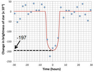
Exercise 22.2 How do we know the sizes of exoplanets?
| Description | Sun | Kepler-452 | Ratio |
|---|---|---|---|
| Temperature (degrees Kelvin) | 5778 | 5757 | 1.0036 |
| Luminosity (x 1026 Watts) | 3.846 | 4.615 | 1.20 |
| Radius (km) | 696,300 | 768,317 |
* The temperatures of the sun and Kepler-452 are very similar, but the small difference is important. Keep 4 decimal places.
| Decrease in brightness* | Earth radius (km) | Kepler-452b radius rplanet (km) | Kepler-452b radius/ Earth radius |
|---|---|---|---|
| 197 x 10-6 | 6378 | 10,784 | 1.7 |
* Because we know this is a decrease, you don’t need to keep the negative sign.
Answers for Chapter 22 were provided by Karla Panchuk.
