9.1 Understanding Earth Through Seismology

Seismology is the study of vibrations within Earth. These vibrations are caused by various events: earthquakes, extraterrestrial impacts, explosions, storm waves hitting the shore, and tidal effects. Of course, seismic techniques have been most widely applied to the detection and study of earthquakes, but there are many other applications, and arguably seismic waves provide the most important information that we have concerning Earth’s interior. Before going any deeper into Earth, however, we need to take a look at the properties of seismic waves. The types of waves that are useful for understanding Earth’s interior are called body waves, meaning that, unlike the surface waves on the ocean, they are transmitted through Earth materials.

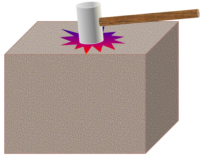
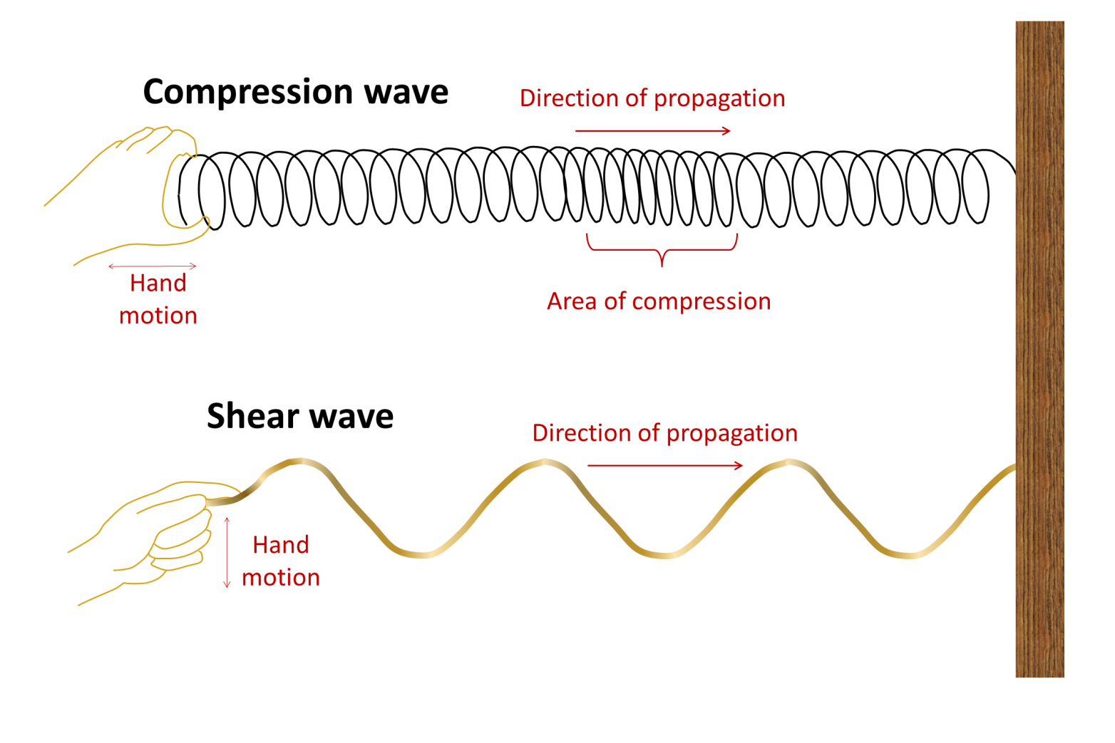
Imagine hitting a large block of strong rock (e.g., granite) with a heavy sledgehammer (Figure 9.1.1). At the point where the hammer strikes it, a small part of the rock will be compressed by a fraction of a millimetre. That compression will transfer to the neighbouring part of the rock, and so on through to the far side of the rock—all in a fraction of a second. This is known as a compression wave, and it can be illustrated by holding a loose spring (like a Slinky) that is attached to something (or someone) at the other end. If you give it a sharp push so the coils are compressed, the compression propagates (travels) along the length of the spring and back (Figure 9.1.2). You can think of a compression wave as a “push” wave—it’s called a P wave (although the “P” stands for “primary” because P waves arrive first at seismic stations).

When we hit a rock with a hammer, we also create a different type of body wave, one that is characterized by back-and-forth vibrations (as opposed to compressions). This is known as a shear wave (S wave, where the “S” stands for “secondary”), and an analogy would be what happens when you flick a length of rope with an up-and-down motion. As shown in Figure 9.1.2, a wave will form in the rope, which will travel to the end of the rope and back.

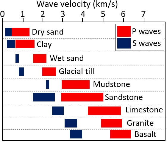
Compression waves and shear waves travel very quickly through geological materials. As shown in Figure 9.1.3, typical P wave velocities are between 0.5 kilometres per second (km/s) and 2.5 km/s in unconsolidated sediments, and between 3.0 km/s and 6.5 km/s in solid crustal rocks. Of the common rocks of the crust, velocities are greatest in basalt and granite. S waves are slower than P waves, with velocities between 0.1 km/s and 0.8 km/s in soft sediments, and between 1.5 km/s and 3.8 km/s in solid rocks.

Mantle rock is generally denser and stronger than crustal rock and both P- and S-waves travel faster through the mantle than they do through the crust. Moreover, seismic-wave velocities are related to how tightly compressed a rock is, and the level of compression increases dramatically with depth. Finally, seismic waves are affected by the phase state of rock. They are slowed if there is any degree of melting in the rock. If the material is completely liquid, P waves are slowed dramatically and S waves are stopped altogether.

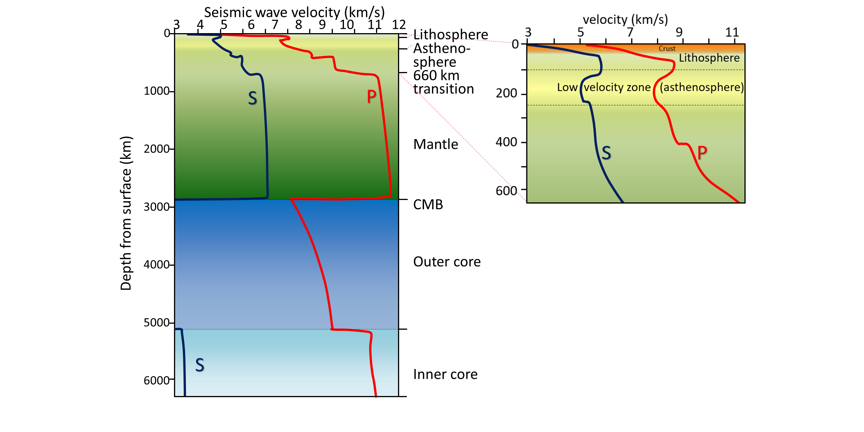
As shown on the right-hand part of Figure 9.1.4, the upper approximately 100 km of the Earth is known as the lithosphere.  This includes the rigid upper part of the mantle (or lithospheric mantle) and the crust.  The next 150 km is the asthenosphere or low velocity zone (because seismic waves are slowed as they pass through that material). As we’ll see below, that part of the mantle is close to it’s melting point and in some regions may be partially molten.

Accurate seismometers have been used for earthquake studies since the late 1800s, and systematic use of seismic data to understand Earth’s interior started in the early 1900s. The rate of change of seismic waves with depth in Earth (as shown in Figure 9.1.4) has been determined over the past several decades by analyzing seismic signals from large earthquakes at seismic stations around the world. Small differences in arrival time of signals at different locations have been interpreted to show that:

• Velocities are greater in mantle rock than in the crust.
• Velocities generally increase with pressure, and therefore with depth.
• Velocities slow in the area between a 100 and 250 kilometre depth (called the “low-velocity zone”; equivalent to the asthenosphere).
• Velocities increase dramatically at 660 kilometre depth (because of a mineralogical transition).
• Velocities slow in the region just above the core-mantle boundary (the D” (d-double-prime) layer or “ultra-low-velocity zone”).
• S waves do not pass through the outer liquid part of the core, but S waves can be created by P waves at the surface of the inner core and their inner core velocity is 3.6 km/s.
• P wave velocities increase dramatically at the boundary between the liquid outer core and the solid inner core.

One of the first discoveries about Earth’s interior made through seismology was in 1909 when Croatian seismologist Andrija Mohorovičić (pronounced Moho-ro-vi-chich) realized that at certain distances from an earthquake, two separate sets of seismic waves arrived at a seismic station within a few seconds of each other. He reasoned that the waves that went down into the mantle, traveled through the mantle, and then were bent upward back into the crust, reached the seismic station first because although they had farther to go, they traveled faster through mantle rock (as shown in Figure 9.1.5). The boundary between the crust and the mantle is known as the Mohorovičić discontinuity (or Moho). Its depth is between  30 and 40 kilometres beneath most of the continental crust, and between 5 and 10 kilometres beneath the oceanic crust.

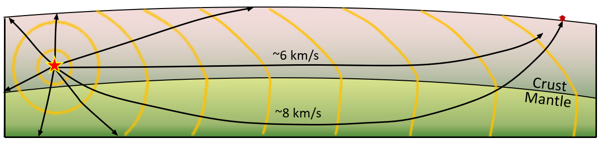
Our current understanding of the patterns of seismic wave transmission through Earth is summarized in Figure 9.1.6. Because of the gradual increase in density (and therefore rock strength) with depth, all waves are refracted (toward the lower density material) as they travel through homogenous parts of Earth and thus tend to curve outward toward the surface. Waves are also refracted at boundaries within Earth, such as at the Moho, at the core-mantle boundary (CMB), and at the outer-core/inner-core boundary.

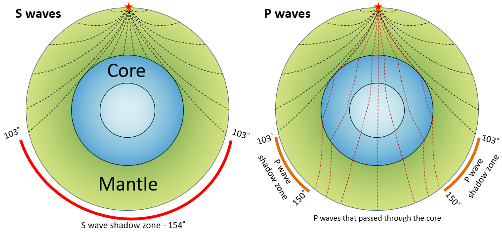
S waves do not travel through liquids—they are stopped at the CMB—and there is an S wave shadow on the side of Earth opposite a seismic source. The angular distance from the seismic source to the shadow zone is 103° on either side, so the total angular distance of the shadow zone is 154°. We can use this information to infer the depth to the CMB.

P waves do travel through liquids, so they can make it through the liquid part of the core. Because of the refraction that takes place at the CMB, waves that travel through the core are bent away from the surface, and this creates a P wave shadow zone on either side, from 103° to 150°. This information can be used to discover the differences between the inner and outer parts of the core.

Exercise 9.2 Liquid Cores in Other Planets

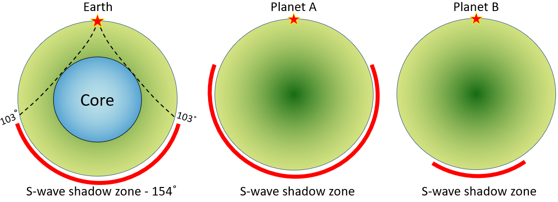
We know that other planets must have (or at least did have) liquid cores like ours, and we could use seismic data to find out how big they are. The S wave shadow zones on planets A and B are shown. Using the same method used for Earth (on the left), sketch in the outlines of the cores for these two other planets.

See Appendix 3 for Exercise 9.2 answers.

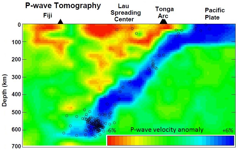
Using data from many seismometers and hundreds of earthquakes, it is possible to create a two- or three-dimensional image of the seismic properties of part of the mantle. This technique is known as seismic tomography, and an example of the result is shown in Figure 9.1.8.

The Pacific Plate subducts beneath Tonga and appears in Figure 9.1.8 as a 100 kilometre thick slab of cold (blue-coloured) oceanic crust that has pushed down into the surrounding hot mantle. The cold rock is more rigid than the surrounding hot mantle rock, so it is characterized by slightly faster seismic velocities. There is volcanism in the Lau spreading centre and also in the Fiji area, and the warm rock in these areas has slower seismic velocities (yellow and red colours).

Image descriptions

[Return to Figure 9.1.3]

[Return to Figure 9.1.4]

Media Attributions

• Figures 9.1.1, 9.1.2, 9.1.4, 9.1.5, 9.1.6, 9.1.7: © Steven Earle. CC BY.
• Figure 9.1.3: “P Wave Velocity, m/s” and “Shear Wave Velocity, m/s” by the US Environment Protection Agency. Edited by Steven Earle. Public domain.
• Figure 9.1.8: “P-wave Tomography” by D. Zhao, Y. Xu, D.A. Wiens, L. Dorman, J. Hildebrand, and S. Webb. (Science, p. 278, 254-257, 1997). Used with permission.