Chapter 14 Groundwater
14.2 Groundwater Flow
If you go out into your garden or into a forest or a park and start digging, you will find that the soil is moist (unless you’re in a desert), but it’s not saturated with water. This means that some of the pore space in the soil is occupied by water, and some of the pore space is occupied by air (unless you’re in a swamp). This is known as the unsaturated zone. If you could dig down far enough, you would get to the point where all of the pore spaces are 100% filled with water (saturated) and the bottom of your hole would fill up with water. The level of water in the hole represents the water table, which is the surface of the saturated zone. In most parts of British Columbia, the water table is several metres below the surface.
Water falling on the ground surface as precipitation (rain, snow, hail, fog, etc.) may flow off a hill slope directly to a stream in the form of runoff, or it may infiltrate the ground, where it is stored in the unsaturated zone. The water in the unsaturated zone may be used by plants (transpiration), evaporate from the soil (evaporation), or continue past the root zone and flow downward to the water table, where it recharges the groundwater.
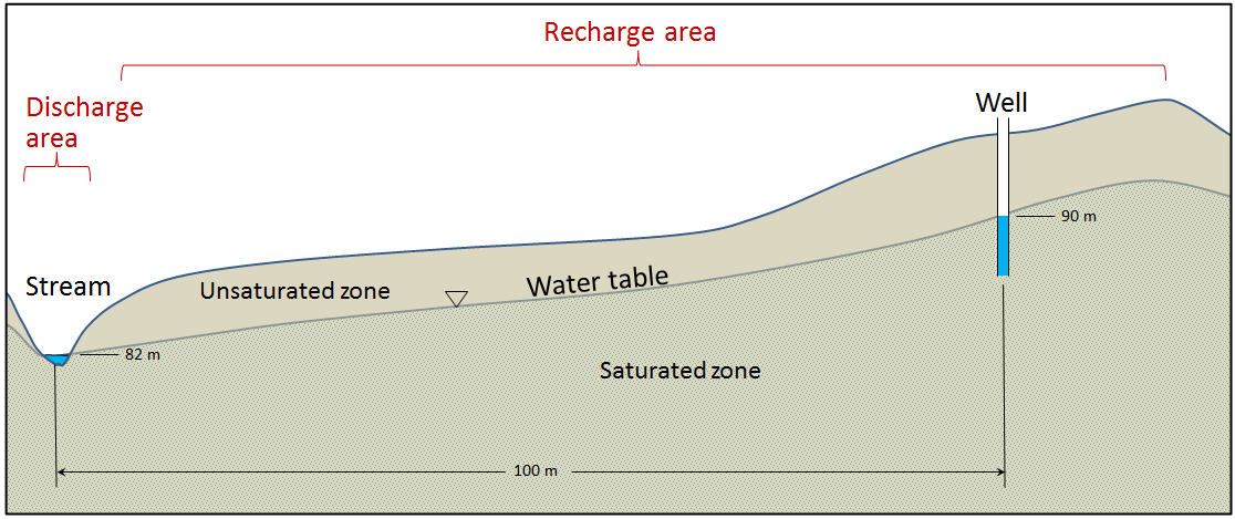
A cross-section of a typical hillside with an unconfined aquifer is illustrated in Figure 14.2.1. In areas with topographic relief, the water table generally follows the land surface, but tends to come closer to surface in valleys, and intersects the surface where there are streams or lakes. The water table can be determined from the depth of water in a well that isn’t being pumped, although, as described below, that only applies if the well is within an unconfined aquifer. In this case, most of the hillside forms the recharge area, where water from precipitation flows downward through the unsaturated zone to reach the water table. The area at the stream or lake to which the groundwater is flowing is a discharge area.
What makes water flow from the recharge areas to the discharge areas? Recall that water is flowing in pores where there is friction, which means it takes work to move the water. There is also some friction between water molecules themselves, which is determined by the viscosity. Water has a low viscosity, but friction is still a factor. All flowing fluids are always losing energy to friction with their surroundings. Water will flow from areas with high energy to those with low energy. Recharge areas are at higher elevations, where the water has high gravitational energy. It was energy from the sun that evaporated the water into the atmosphere and lifted it up to the recharge area. The water loses this gravitational energy as it flows from the recharge area to the discharge area.
In Figure 14.2.1, the water table is sloping; that slope represents the change in gravitational potential energy of the water at the water table. The water table is higher under the recharge area (90 metres) and lower at the discharge area (82 metres). Imagine how much work it would be to lift water 8 metres high in the air. That is the energy that was lost to friction as the groundwater flowed from the top of the hill to the stream.
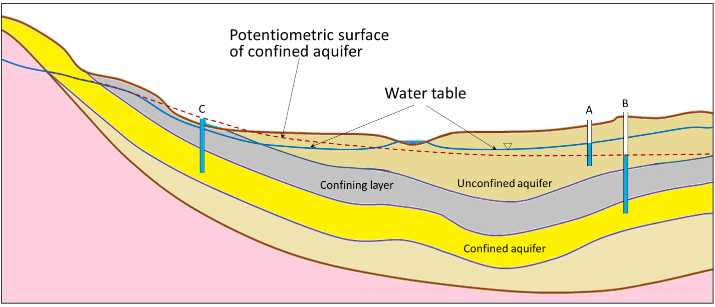
The situation gets a lot more complicated in the case of confined aquifers, but they are important sources of water so we need to understand how they work. As shown in Figure 14.2.2, there is always a water table, and that applies even if the geological materials at the surface have very low permeability. Where there is a confined aquifer — meaning one that is separated from the surface by a confining layer — this aquifer will have its own “water table,” which is actually called a potentiometric surface, as it is a measure of the total potential energy of the water. The red dashed line in Figure 14.2.2 is the potentiometric surface for the confined aquifer, and it describes the total energy that water is under within the confined aquifer. If we drill a well into the unconfined aquifer, the water will rise to the level of the water table (well A in Figure 14.2.2). But if we drill a well through both the unconfined aquifer and the confining layer and into the confined aquifer, the water will rise above the top of the confined aquifer to the level of its potentiometric surface (well B in Figure 14.2.2). This is known as an artesian well, because the water rises above the top of the aquifer. In some situations, the potentiometric surface may be above the ground level. The water in a well drilled into the confined aquifer in this situation would rise above ground level, and flow out, if it’s not capped (well C in Figure 14.2.2). This is known as a flowing artesian well.
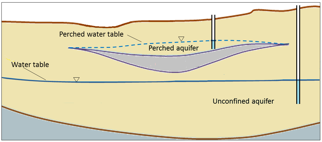
In situations where there is an aquitard of limited extent, it is possible for a perched aquifer to exist as shown in Figure 14.2.3. Although perched aquifers may be good water sources at some times of the year, they tend to be relatively thin and small, and so can easily be depleted with over-pumping.
In 1856, French engineer Henri Darcy carried out some experiments from which he derived a method for estimating the volume of groundwater flow based on the hydraulic gradient and the permeability of an aquifer, expressed using K, the hydraulic conductivity. Darcy’s equation, which has been used widely by hydrogeologists ever since, looks like this:
[latex]Q=K\times i \times A[/latex]
where Q is the volume of the groundwater flow (m3/s), K is the hydraulic conductivity (m/s), i is the hydraulic gradient, and A is the cross-sectional area of the aquifer.
The following equation can be used to determine the flux (i.e., volume per unit time) of groundwater passing through the area of the aquifer being considered. This is how much groundwater flows through each unit area of aquifer:
[latex]q=\dfrac{Q}{A}=K\times i[/latex]
Lower-case q is known as the Darcy flux; it typically has units of metres per second (although other units can be used, such as cm/day or ft/minute). It is not the velocity of the groundwater, but is a description of how much volume (m3/s) passes through each area (m2), so the typical units are [latex]\dfrac{m^3/ \text{s}}{m^2}[/latex]. In reality, the groundwater does not pass through all of the cross-sectional area of the aquifer (A): it can only pass through the pores. The actual velocity of the water is how fast the water must move through the pores in order to get the same flux — [latex]\dfrac{m^3/ \text{s}}{m^2}[/latex] — through the open area (total area × porosity). So the equation to estimate flow velocity is as follows:
[latex]V=\dfrac{K\times i}{n}[/latex]
where V is the velocity of the groundwater, and n is the porosity (expressed as a proportion, so if the porosity is 10%, n = 0.1).
We can apply this equation to the scenario in Figure 14.2.1. If we assume that the hydraulic conductivity is 0.00001 metres per second (m/s), we get q = 0.00001 × 0.08 = 0.0000008 m3 per second per m2. If the material has a porosity of 25%, then the true velocity of the groundwater is:
[latex]V=\dfrac{q}{n}=\dfrac{0.0000008\text{ m/s}}{0.25}=0.0000032\text{ m/s}[/latex]
That is equivalent to 0.000192 metres/minute, 0.0115 metres/hour or 0.276 m/day. That means it would take 361 days for water to travel the 100 metres from the vicinity of the well to the stream. Groundwater moves slowly, and that is a reasonable amount of time for water to move that distance. In fact, it would likely take longer than that, because it doesn’t travel in a straight line.
Exercise 14.1 How long will it take?

Sue, the owner of Joe’s 24-Hour Gas, has discovered that her underground storage tank (UST) is leaking fuel. She calls in a hydrogeologist to find out how long it might take for the fuel contamination to reach the nearest stream. They discover that the well at Joe’s has a water level that is 37 metres above sea level and the elevation of the stream is 21 metres above sea level. The sandy sediment in this area has a permeability (K) of 0.0002 metres per second and a porosity of 25% (n = 0.25).
Using [latex]V=\dfrac{K\times i}{n}[/latex], estimate the velocity of groundwater flow from Joe’s to the stream, and determine how long it might take for contaminated groundwater to flow the 80 metres to the stream.
See Appendix 3 for Exercise 14.1 answers.
It’s critical to understand that groundwater does not flow in underground streams, nor does it form underground lakes. With the exception of karst areas, with caves in limestone, groundwater flows very slowly through granular sediments, or through solid rock that has fractures in it. Flow velocities of several centimetres per day are possible in significantly permeable sediments with significant hydraulic gradients. But in many cases, permeabilities are lower than the ones we’ve used as examples here, and in many areas, gradients are much lower. It is not uncommon for groundwater to flow at velocities of a few millimetres to a few centimetres per year.
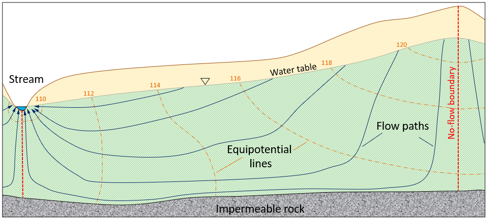
As already noted, groundwater does not flow in straight lines. It flows from areas of higher hydraulic head to areas of lower hydraulic head, and this means that it can flow “uphill” in many situations. This is illustrated in Figure 14.2.5. The dashed orange lines are equipotential lines, meaning lines of equal pressure. The blue lines are the predicted groundwater flow paths. Note that in some areas the groundwater will flow steeply down, in other areas it will flow down only at a shallow angle, and in some areas—especially near to discharge zones—it will flow upward. The dashed red lines are no-flow boundaries, meaning that water cannot flow across these lines. That’s not because there is something there to stop it, but because there’s no pressure gradient that will cause water to flow in that direction.
Groundwater flows at right angles to the equipotential lines in the same way that water flowing down a slope would flow at right angles to the contour lines. The stream in this scenario is the location with the lowest hydraulic potential, so the groundwater that flows to the lower parts of the aquifer has to flow upward to reach this location. It is forced upward by the pressure differences, for example, the difference between the 112 and 110 equipotential lines.
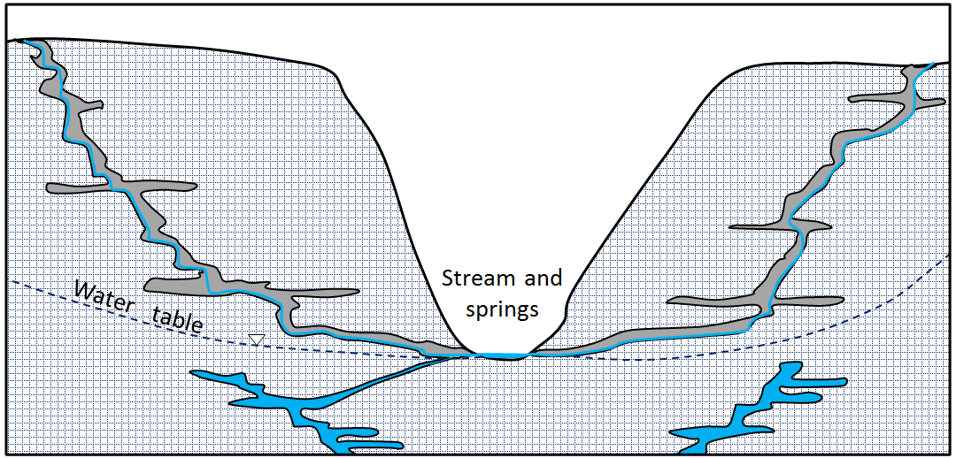
Groundwater that flows through caves, including those in karst areas—where caves have been formed in limestone because of dissolution—behaves differently from groundwater in other situations. Caves above the water table are air-filled conduits, and the water that flows within these conduits is not under pressure; it responds only to gravity. In other words, it flows downhill along the gradient of the cave floor (Figure 14.2.6). Many limestone caves also extend below the water table and into the saturated zone. Here water behaves in a similar way to any other groundwater, and it flows according to the hydraulic gradient and Darcy’s law.
Image Descriptions
Figure 14.2.2 image description: A cross-section showing three layers. The top layer is an unconfined aquifer. A well has been drilled into the unconfined aquifer and filled up to the height of the water table. Below the unconfined aquifer is a confining layer, and below that is a confined aquifer. A well has been drilled through the confining layer and into the confined aquifer. Water fills that well up to the potentiometric surface of the confined aquifer, which, in this case, is above the confining layer. [Return to Figure 14.2.2]
Media Attributions
- Figure 14.2.1, 14.2.3, 14.2.4, 14.2.5, 14.2.6: © Steven Earle. CC BY.
the rock or sediment above the water table
the upper surface of the saturated zone in an unconfined aquifer
the part of an aquifer, or any body of rock, that is saturated with water
flow of water down a slope, either across the ground surface, or within a series of channels
the recharge of groundwater from the downward percolation of surface water
the transfer of surface water into the ground to become groundwater
an area of an aquifer where recharge is predominant over discharge
the part of an aquifer where groundwater discharge takes place
the imaginary surface defined by the levels to which water would rise in a series of wells drilled into a confined aquifer
a well that is completed in a confined aquifer and in which the water level in the well rises above the top of the aquifer
an artesian well in which the water level naturally rises above the surface of the ground
the solutional erosion of an area with soluble rock (typically limestone) to form depressions and caves
in the context of groundwater an equipotential line connects locations with equal hydraulic head or water pressure
the path that groundwater flows along between a recharge area and a discharge area
