8 Data Analysis 2
8.4 Z-Scores and the Normal Curve

Learning Objectives
By the end of this section it is expected that you will be able to:
- Convert a data item to a z-score
- Solve applications using z-score tables
The Normal Curve
When a set of data values is normally distributed, the 68-95-99.7 Rule can be used to determine the percentage of values that lie one, two or three standard deviations from the mean. We will shift gears and explore how to determine where a specific data value lies in relation to all other values. As an example, a student who has written a college entrance exam may want to know where they placed in comparison to all other students. This section will explore how to determine this.
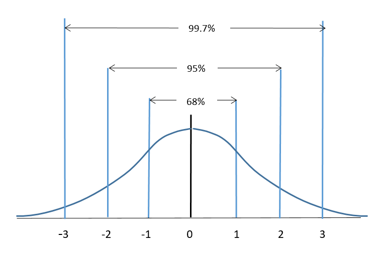
Consider the normal curve which is an idealized representation of a normally distributed population. The normal curve, also called a bell-shaped curve, is represented in Figure 1. The area under the curve represents 100% (or 1.00) of the data (or population) and the mean score is 0.

We have seen that the standard deviation plays an important role in the normal distribution.
Refer to Figure 2 for the visual representation of the 68 – 95 – 99.7 Rule. For a normally distributed set of data:
- Approximately 68% (68.26%) of the data items fall within one standard deviation of the mean.
- Approximately 95% (95.44%) of the data items fall within two standard deviations of the mean.
- Approximately 99.7% of the data items fall within three standard deviations of the mean.

Z–Scores
When a data set is normally distributed we can use a standardized score, called the z-score, to determine the number of standard deviations that a data value is from the mean.
Reconsider an example from the previous section. Acertain segment of the economy has a normally distributed salary, with a mean salary of $45,000 and a standard deviation of $4000. Refer to Figure 3.
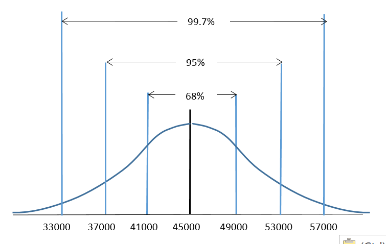
With this information we are able to determine that a salary of $49,000 lies exactly one standard deviation above the mean since $45,000 + $4000 = $49, 000. In turn, using the 68-95-99.7 Rule we can determine that a salary of $49,000 is higher than 84% of the other salaries for this segment of the economy. The calculation would be 50% + (68%/2) = 84%. This calculation was possible since $49,000 was exactly one standard deviation away from the mean.
Consider a salary which does not lie exactly one, two or three standard deviations from the mean, such as $38,500. The calculation does not appear so straightforward but as it turns out we can use a z-score for situations such as this. A z-score converts a data value and standardizes it so that we are able to determine how many standard deviations a specific data value will lie above or below the mean.
Z-scores can be used in situations with a normal distribution. Consider a chemistry class with a set of test scores that is normally distributed. The average score is 76% and one student receives a score of 55%. Converting the 55% to a z-score will provide the student with a sense of where their score lies with respect to the rest of the class. We can also use z-scores to determine the percent of the data values that will lie between any two data values. Perhaps we wish to determine the percentage of students whose test scores lie between 70% to 85%. This can also be done using z-scores.
We have seen that when calculating standard deviation we must consider whether we are working with the entire population or a sample of the population. We must do the same when calculating a z-score.
Formulas for Finding Z-Scores
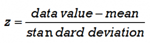
The z-score represents the number of standard deviations a data value is from the mean value.
The formula for z is:
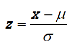
For a population we calculate the z-score using the population mean μ and standard deviation σ. The data value is represented by x.
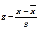
For a representative sample of the population we calculate the z-score using the sample mean and standard deviation.:
A z-score is similar to a percentile in that it is a measure of position. As a rule, z-scores above 2.0 (or below –2.0) are considered “unusual” values. According to the 68-95-99.7 Rule, in a normal population such scores would occur less than 5% of the time. Z-scores between -2.0 and 2.0 are considered “ordinary” values and these represent 95% of the values.
EXAMPLE 1
IQ scores are normally distributed. The mean IQ is 100 and the standard deviation is 15.
a) If Frank has an IQ of 127, find his z-score. b) Intrepret the meaning of this z-score. c) Using the 68-95-99.7 Rule, how does Frank’s IQ compare to the rest of the population?
Solution
a) We will use the z-score for a population:
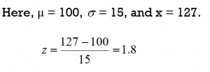
Frank’s z-score is 1.8.
b) For this z-score, the mean of 100 has been “standardized” to a value of 0 and the score of 127 has been standardized to a value of 1.8. This means that Frank’s IQ score is 1.8 (almost 2 standard deviations) higher than the average.
c) Considering the 68-95-99.7 Rule, Frank’s score lies within 2 standard deviations of the mean. His score is certainly better than at least 84% of the population but does not rank in the top 2.5% of the population.
TRY IT 1
Consider a chemistry class and a set of test scores with an average of 76% and a standard deviation of 7%. A student receives a test score of 55%. a) Determine the student’s z-score. b) Intrepret the meaning of this z-score. c) Using the 68-95-99.7 Rule, how does the student’s test score compare to the rest of the class?
Show answer
a) z-score = -3 b) This z-score is exactly 3 standard deviations less than the mean score of 76%. c) This student scored better than only 0.15% of the class (or 99.85% of the class scored higher than this student).
In Example 1 we were able to determine that Frank’s score is better than at least 84% of the population but it does not rank in the top 2.5% of the population. This is a fairly broad conclusion. As it turns out we can be more specific if we use z-score tables.
Z-Score Tables
A z-score table allows us to determine, for a normal distribution, the percentage of data values that lie below (to the left) of a specific z–score. This in turn will enable us to determine the percentage of values that lie between or to the right of a given z-score.
We will use two different z-tables, one for positive z-scores and one for negative z-scores. These tables are available online (or refer to the Tables at the end of this chapter).
A portion of a positive z-score table is shown in Figure 4. We use the positive z-table when we have z-scores that are greater than 0 or lie to the right of the mean. The number in the z-table represents the area under the bell curve to the left of the z-score. The number is stated as a decimal fraction which can then be converted to a percentage by multiplying by 100. If for example the number in the table is 0.62552, then this would be interpreted as 62.552%.

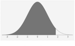
Consider a data value X that is found to have a standardized z-score of 1.42. A data value with a z-score of 1.42 will lie between 1 and 2 standard deviations above the mean (refer to Fig. 5). We can use a z-zcore table to determine the proportion of data vales that are less than (or geater than) this score.
This z-score value of 1.42 is positive so we refer to the positive z-score table in Figure 4. In the table go down the first column until you reach +1.4. The first column provides the z-score values to the nearest tenth (or one decimal place). To incorporate the digit that is in the second decimal place we must move through the body of the table until the heading of the column matches the digit in the hundredths place. In this example we move across the row for +1.4 until we reach the column headed with a 0.02. The corresponding number in the table is 0.92220 so for a z-score of 1.42 we can state that the area to the left of this score is 0.92220. Alternatively, 92.220% of all data values are less than this data value X. We are also able to conclude that 7.8% of the data values lie above this z-score value since 100% – 92.2% = 7.8%
Using only the z-score of 1.42 we were able to conclude that the data value X will lie between 1 and 2 standard deviations above the mean. By using the z-score table we are able to be more specific in stating that approximately 92% of the data values are less than X.
EXAMPLE 2
Consider a z-score of 0.18. a) Determine the area under the curve for a z-score of 0.18. b) Interpret what this z-score tells us.
Solution
a) This value is positive so we refer to the positive z-score table (a partial table is provided in Figure 4). In the table go down the first column until you reach +0.1. Then move across the row until you reach the column headed with a 0.08. This represents a z-score of 0.18. For a z-score of 0.18 the number in the table is 0.57142.
b) For a data value with a z-score of 0.18, approximately 57.1% of the data values will be below this and 42.9% will be above this data value.
TRY IT 2
Consider a z-score of 0.90. a) Determine the area under the curve for a z-score of 0.90. b) Interpret what this z-score tells us.
Show answer
a) area is 0.81594 b) Approximately 81.6% of data values are less than this value (or 18.4% are greater).
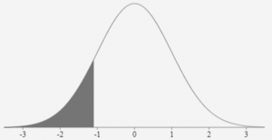
If the z-score is negative we use a negative z-table, a portion of which is illustrated in Figure 6. This table provides z-scores that are less than 0 or lie to the left of the mean. The number in the z-table represents the area under the bell curve to the left of the z-score.

Consider an observation that has a z-score of -1.17. Refer to the negative z-score table in Figure 6. In the table go down the first column until you reach -1.1. Then move across the row until you reach the column headed with a 0.07. For a z-score of -1.17 the number in the table is 0.12100 or 12.1%. This represents the portion of the data values that lie to the left of the z-score (refer to Figure 7). This means that 12.1% of the data values are less than this data value. Alternatively 87.9% (100% – 12.1%) of the data values are greater than this data observation.
Z-Scores and the 68-95-99.7 Rule
With a normal distribution half of the data values lie below the mean and half lie above the mean. If we calculate the z-score for a mean of 0 we will find that the z-score will also be 0. From the z-table we can determine that for a z-score of 0 the number is 0.5. This indicates that 50% of the data values lie below the mean and therefore 50% of the data values lie above the mean.
Refer to the normal distribution that is illustrated in Figure 8. For standard deviations of 1, 2 or 3 we can use the 68-95-99.7 Rule to determine areas under the curve. We can also use z-score tables to do this.
EXAMPLE 3
a) A data value X is found to lie -1 standard deviation from the mean. Use the 68-95-99.7 Rule to determine the percentage of data values that are lower than this data value.
b) For a data value X with a z-score of -1, determine the percentage of data values that are lower than X.
Solution
a) Refer to Figure 8. If 68% of the data values lie between -1 and 1 standard deviations, then 100% – 68% = 32% lie on either side of -1 or 1 standard deviations from the mean. Dividing 32% in half we get 16%. Therefore 16% of all data values are lower than the data value X. (Note: There are other approaches to this calculation).
b) Refer to the negative z-score table in Figure 6. For a z-score of -1 the area will be 0.15866 or 15.866%. Rounded to the nearest whole number we determine that 16% of the data values are lower than this data value.
Note: The z-score table will provide more accurate results than the 68-95-99.7 Rule since the values in the 68-95-99.7 Rule are rounded off approximations.
TRY IT 3
a) A data value X is found to lie 3 standard deviations from the mean. Use the 68-95-99.7 Rule to determine the percentage of data values that are greater than this data value.
b) For a data value X with a z-score of 3, determine the percentage of data values that are greater than X.
Show answer
a) Refer to Figure 8. If 99.7% of the data values lie between -3 and 3 standard deviations, then 100% – 99.7% = 0.3% lie on either side of -3 or 3 standard deviations from the mean. Dividing 0.3% in half we get 0.15%. Therefore 0.15% of all data values are greater than the data value X.
b) Refer to a positive z-score table. For a z-score of 3 the area to the left will be 0.99865 or 99.865% so the area to the right (greater) will be 100% – 99.865% = 0.135% Rounded to the nearest 2 decimal places we determine that 0.14% of the data values are greater than this data value. Note that this slightly different than the answer obtained from using the 68-95-99.7 Rule due to rounding.
Areas Between Z-Scores
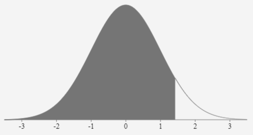
We can use z-score tables to determine the area between two z-scores. As an example, we can use the table to determine the area between the mean and a z-score of 1. A z-score of 1 lies one standard deviation to the right of the mean (as in Figure 9). Refer to the positive z-table in Figure 4. For a z-zcore of 1 the value in the table is 0.84134. This indicates that approximately 84% of the data values lie to the left of this z-score.
From the z-score table we determine that for the z-score of 0 the area to the left is 0.5000. The area between the mean and one standard deviation would be as follows:
0.84134 – 0.500 = 0.3413 or 34.13%
Figure 10 illustrates the area between the mean and one standard deviation.
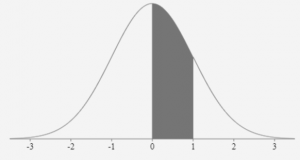
Note that this is consistent with the 68-95-99.7 Rule. It states that approximately 68% of the data will lie within one standard deviation on either side of the mean. Half this amount, or 34%, will lie between the mean and a standard deviation of one.
The 68-95-99.7 Rule is useful when data values lie exactly 1, 2 or 3 standard deviations from the mean. Z-score tables are useful for data values that have z-scores that are not exactly 1, 2 or 3 standard deviations from the mean.
EXAMPLE 4
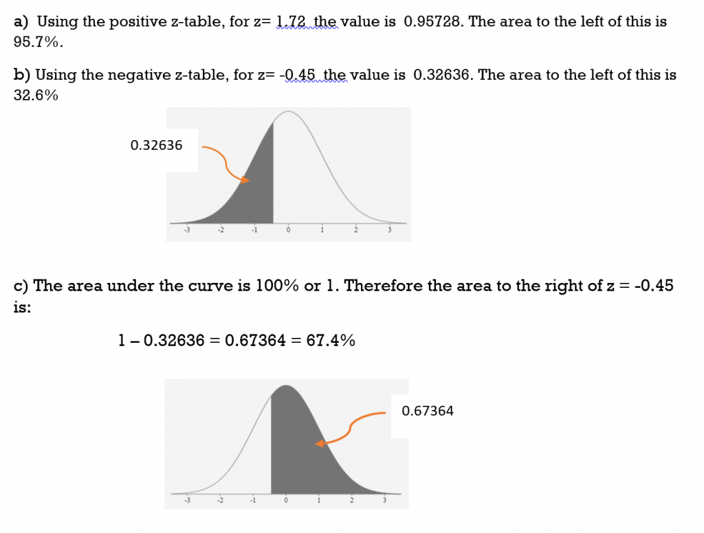
Given a normal distribution, use the z-score tables to find the area for each of the following z-scores (rounded to the nearest tenth of a percent):
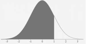
a) to the left of z = 1.72
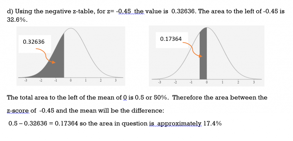
b) to the left of z = -0.45
c) to the right of z = -0.45
d) between -0.45 and the mean
Solution
TRY IT 4
Given a normal distribution, find the area for each of the following z-scores (rounded to the nearest tenth of a percent):
a) to the left of z = 0.85
b) to the right of z = 0.85
c) between the mean and z = 0.85
Show answer
a) 0.8023 = 80.2%
b) 0.1977 = 19.8%
c) 0.8023 – 0.5 = 0.3023 = 30.2%
EXAMPLE 5
Given a normal distribution, find the area for each of the following z-scores (rounded to the nearest tenth of a percent):
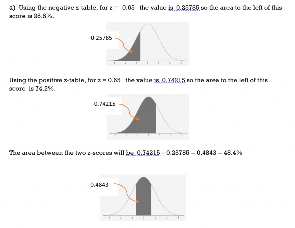
a) between z = -0.65 and z = 0.65
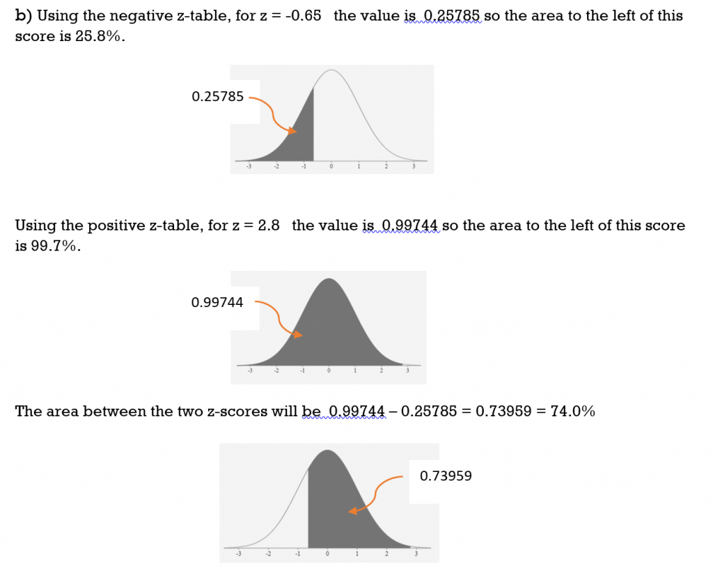
b) between z = -0.65 and z = 2.8
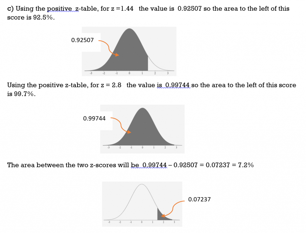
c) between z = 1.44 and z = 2.8
Solution
TRY IT 5
Given a normal distribution, find the area for each of the following z-scores (rounded to the nearest tenth of a percent):
a) between z = 0 and z = -0.73
b) between z = -0.73 and z = 1.95
c) between z = -2.12 and z = -0.73
Show answer
a) 0.2673 = 26.7%
b) 0.7417 = 74.17%
c) 0.2157 = 21.6%
Applications Using Z-Scores
With populations or samples that are normally distributed, z-scores can be used to determine how data values compare (are positioned) with respect to other data values.
EXAMPLE 6
Frank has an IQ of 127, or a z score of 1.8. What percent of the population have IQ scores less than 127 and what percent have IQ scores higher than 127?
Solution
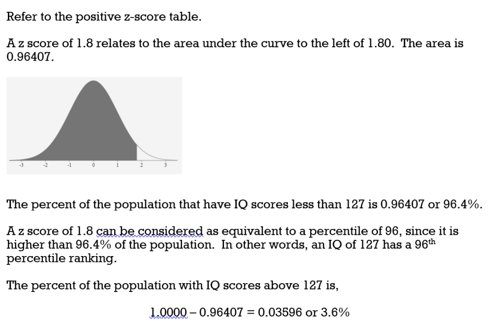
Refer back to Example 1 where the 68-95-99.7 Rule was used to analyze Frank’s IQ score. From the Rule we were able to conclude that Frank’s IQ was better than at least 84% of the other scores and that his score did not rank in the top 2.5%. Comparing the two methods, the z-score provides us with a much more accurate analysis.
TRY IT 6
Consider a chemistry class and a set of test scores with an average of 76% and a standard deviation of 7%. A student receives a test score of 55% which yields a z-score of -3 (refer to TRY IT 1). a) Use a z-score table to determine what percent of the class had test scores less than 55% and what percent had test scores greater than 55%. b) How does this compare with the answer to TRY IT 1?
Show answer
a) From the table the area to the left of a z-score of -3 is 0.00135 therefore 0.135% of the class had test scores less than 55% and 99.865% of the class scored higher than 55%. b) Using the Rule in TRY IT1 the results were slightly different due to rounding: 0.15% of the students scored less than 55% and 99.85% scored higher than 55%.
For applications involving populations or samples that are normally distributed, we can calculate z-scores if we know the mean and the standard deviation.
EXAMPLE 7
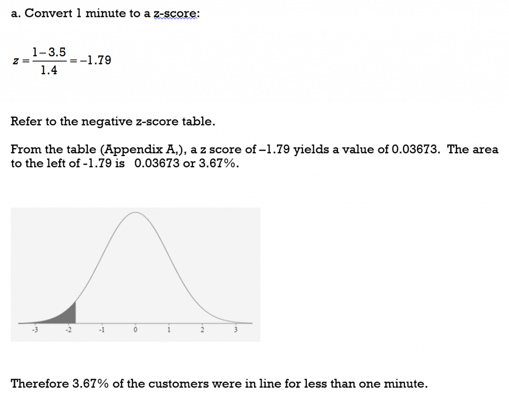
The waiting-in-line time at a certain grocery store is normally distributed with a mean
of 3.5 minutes and a standard deviation of 1.4 minutes.
a) What percent of the customers wait in line less than one minute?
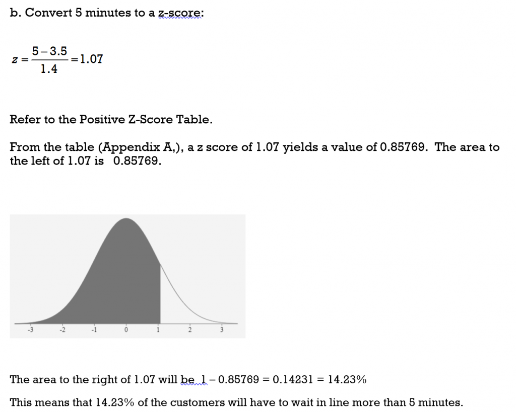
b) What percent of the customers wait in line more than 5 minutes?
Solution
TRY IT 7
The waiting-in-line time to be seated at a popular retaurant during primetime hours is normally distributed with a mean of 24 minutes and a standard deviation of 11 minutes.
a) What percent of the customers wait in line less than twenty minutes?
b) What percent of the customers wait in line more than forty-five minutes?
Show answer
a) 36% of customers wait less than 20 minutes b) 3% of customers wait more than 45 minutes
EXAMPLE 8
All first year psychology students wrote an exam that had 92 questions. Each question was worth 1 point for a total possible 92 points. The marks were normally distributed with a mean of score of 58 points and a standard deviation of 11 points.
a) Determine the z-score for a mark of 45 points. What percent of the scores were less than 45 points?
b) Determine the z-score for a mark of 84 points. What percent of the scores were greater than 84 points?
c) What percent of the scores were between 76 and 88 points?
Solution:
a) z = -1.1818 and area to the left is 0.11900 so 11.9% of the scores would be less than 45 points
b) z = 2.3636 and the area to the left is 0.99086 so the area to the right is 1- 0.99534 = 0.00914. Therefore 0.9% (almost 1%) would score higher than 84 points
c) for 76 points z = 1.64 and the area to the left is 0.9495. For 88 points z = 2.73 and the area to the left is 0.99683. The difference is 0.99683 – 0.9495 = 0.04733. This means that 4.7% of the students would score between 76 and 88 points.
TRY IT 8
An entrance exam was given to a cohort of students. The mean score was 1000 points with a standard deviation of 150 points.
a) What percent of the students scored less than 820 points?
b) What percent of the students scored more than 1330 points?
c) What percent of the students scored between 950 and 1100 points?
Show answer
a) 11.5% scored less than 820 points b) 1.4% scored more than 1330 points
c) 37.8% scored between 950 and 1100 points
Key Concepts
- For a population we calculate the z-score for a data value x using the population mean μ and standard deviation σ.
- For a representative sample of the population we calculate the z-score for a data value x using the sample mean and standard deviation. :
- A z-score table allows us to determine, for a normal distribution, the percentage of data values that lie below (to the left) of a specific z–score. This in turn will enable us to determine the percentage of values that lie between or to the right of a given z-score.
- When a z-score is negative (lies to the left of the mean) we use a negative z-score table. When a z-score is positive (lies to the right of the mean) we use a positive z-score table.
Glossary
Z-score
is a standardized score that has been converted from a data value. The z-score indicates how many standard deviations away from the mean a data value lies.
8.4 Exercise Set
- Heights of adult males are normally distributed. The mean height of an adult male is 178 cm with a standard deviation of 10 cm.
- If Matt is 188 cm tall, find his z-score.
- Intrepret the meaning of this z-score.
- Using the 68-95-99.7 Rule, how does Matt’s height compare to the rest of the population?
- Heights of adult males are normally distributed. The mean height of an adult male is 178 cm with a standard deviation of 10 cm.
- If Keegan is 158 cm tall, find his z-score.
- Interpret the meaning of this z-score.
- Using the 68-95-99.7 Rule, how does Keegan’s height compare to the rest of the population?
-
- A data value X is found to lie -3 standard deviations from the mean. Use the 68-95-99.7 Rule to determine the percentage of data values that are less than this data value.
- For a data value X with a z-score of -3, use a negative z-score table to determine the percentage of data values that are lower than X.
-
- A data value X is found to lie 2 standard deviations from the mean. Use the 68-95-99.7 Rule to determine the percentage of data values that are lower than this data value.
- For a data value X with a z-score of 2, use a positive z-score table to determine the percentage of data values that are lower than X.
- Find the area under the normal curve for the followed z scores. Give the answers as both a decimal fraction (as a stated in the z-table) and as a percentage (rounded to the nearest tenth).
- less than z = -0.86 _____________________
- greater than z = -0.86 _____________________
- less than z = 1.34 _____________________
- greater than z = 1.34 _____________________
- greater than z = -2.88 _____________________
- Find the area under the normal curve for the following z scores. Give the answers as both a decimal fraction (as stated in the z-table) and as a percentage (rounded to the nearest tenth).
- between z = 0 and z = 0.47 _____________________
- between z = -0.3 and z = 0 _____________________
- between z = -0.3 and z = 0.47 _____________________
- between z = -2.24 and z = -0.55 _____________________
- between z = 1.46 and z = 2.37 _____________________
- between z = -1.5 and z = 1.5 _____________________
- The average resting heartrate for a normally distributed population of men was found to be 62 beats per minute with a standard deviation of 11 beats per minutes.
- What percent of men have resting heartrates under 70 beats per minute?
- What percent of men have resting heartrates over 70 beats per minute?
- What percent of men have resting heartrates between 40 and 80 beats per minute?
- In a group of normally distributed women, the average height is 5 feet 4 inches (64 inches) with a standard deviation of 2.8 inches. (1 foot = 12 inches)
- What percent of women are shorter than 5 feet?
- What percentage of woman are taller than 6 feet ?
- What percent of the women are between 5 feet and 6 feet ?
- A survey of college students enrolled in technology programs indicated that they spend an average of 29 hours a week outside of class time studying for their courses. The data was normally distributed with a standard deviation of 9 hours per week.
- What percent of the students spend more than 40 hours per week studying?
- What percent spend fewer than 10 hours per week studying?
- What percent spend between 20 and 50 hours per week studying?
- The number of toy cars assembled each day by a worker is normally distributed with a mean of 270 cars and a standard deviation of 16 cars.
- What percentage of workers assemble less than 240 cars per day?
- What percentage of workers assemble more than 265 cars per day?
- Workers are given a bonus every time they assemble more than 310 toy cars in one eight hour day. What percent of the workers receive a bonus each day?
- A radar unit measures the speed of passing cars on a toll highway where the speed limit is 120/km/hour. The speed of the cars is normally distributed with a mean speed of 114 km/h and a standard deviation of 9.8 km/h.
- What percent of the cars are travelling at less than 100 km/h?
- What percent of the vehicles are exceeding the speed limit?
- What percent of the vehicles are travelling between 115 km/h and 125 km/h?
- The lengths of cell phone calls in a particular city are normally distributed with a mean time of 8.2 minutes and a standard deviation of 2.6 minutes.
- What percent of phone calls are less than 10 minutes?
- What percent of phone calls are greater than 5 minutes?
- What percent of phone calls are between 7 and 12 minutes?
Answers
-
- z-score = 1
- This height is one standard deviation greater than the mean
- This height is greater than 84% of the population
-
- z-score = -2
- This height is two standard deviations less than the mean
- Keegan’s height is greater than approximately 2.5% of the population
-
- From the Rule approximately 1.5%
- From the table 1.4%
-
- From the Rule approximately 97.5%
- From the table 97.7%
-
- 0.19489 = 19.5%
- 0.80511 = 80.5%
- 0.90988 = 91.0%
- 0.09012 = 9.0%
- 0.99801 = 99.8%
-
- 0.18082 = 18.1%
- 0.11791 = 11.8%
- 0.29873 = 27.9%
- 0.06326 = 6.3%
- 0.86638 = 86.6%
-
- 76.7%
- 23.3%
- 92.7%
-
- 7.6%
- 0.2%
- 92.2%
-
- 11.1%
- 1.7%
- 83.1%
-
- 3%
- 62.2%
- 0.6%
-
- 7.7%
- 27.1%
- 32.9%
-
- z = 0.6923 and area to the left is 0.75490 so 75.5% of the calls would be less than 10 minutes.
- z = -1.23 and area to the left is 0.10935 so area to the right is 1- 0.10935 = 0.89065 Therefore 89.1% of the calls would be more than 10 minutes.
- 7 minutes has z = -0.4615 and the area to the left is 0.32276 and for 12 minutes z = 1.4615 and the area to the left is 0.92785. The difference is 0.92785 – 0.32276 = 0.60509. This means that 60.5% of the calls would be between 7 and 12 minutes.
Attribution
- Figure 6 is from https://www.ztable.net/.
- Some of the content for this chapter is from “Unit 9: Mortgages”, “Unit 10: Interest rates on loans”, and “Review Questions” in Financial Mathematics by Paul Grinder, Velma McKay, Kim Moshenko, and Ada Sarsiat, which is under a CC BY 4.0 Licence.. Adapted by Kim Moshenko. See the Copyright page for more information.
