8 Data Analysis 2
8.3 The Normal Curve
. Please attribute as Matemateca (IME/USP)/Rodrigo Tetsuo Argenton. This file was published as the result of a partnership between Matemateca (IME/USP), the RIDC NeuroMat and the Wikimedia Community User Group Brasil")
Learning Objectives
After completing this section the student should be able to:
- Recognize the characteristics of a normal distribution
- Find scores at a designated standard deviation from the mean
- Interpret and use the 68-95-99.7 Rule
The Normal Distribution
The Galton Board, invented by Sir Francis Galton, consists of a vertical board with interleaved rows of pegs. Beads are dropped from the top and, when the device is level, bounce either left or right as they hit the pegs. Eventually they are collected into bins at the bottom, where the height of bead columns accumulated in the bins approximate a normal distribution. (https://en.wikipedia.org/wiki/Bean_machine#/)
In this section we will explore the normal distribution and the dispersion of data values around the mean. We have seen that the standard deviation provides a measure of the dispersion of the data values around the mean. If the standard deviation is zero then all data vales will equal the mean. The general idea seems to be that as the standard deviation increases the data will be more widely dispersed around the mean. We have also seen that data can be distributed in a variety of ways. Consider the histograms in Figures 1, 2 & 3. These histograms represent the evaluation scores (on a scale of 1 to 5) for three instructors. In all three cases a group of 10 students provided feedback for each of the instructors.
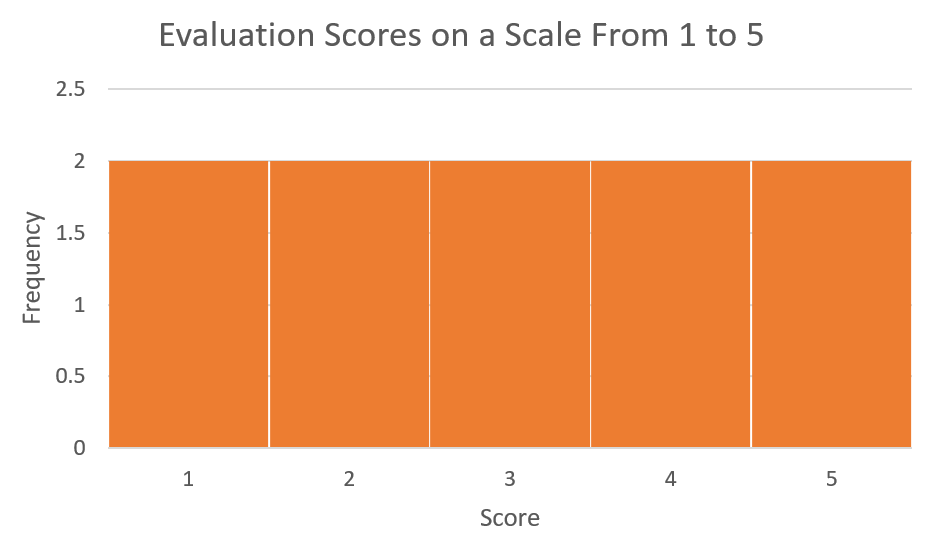
Referring to Figure 1, Instructor A received each possible score two times. Figure 1 represents a uniform distribution since every data value occurs with the same frequency.
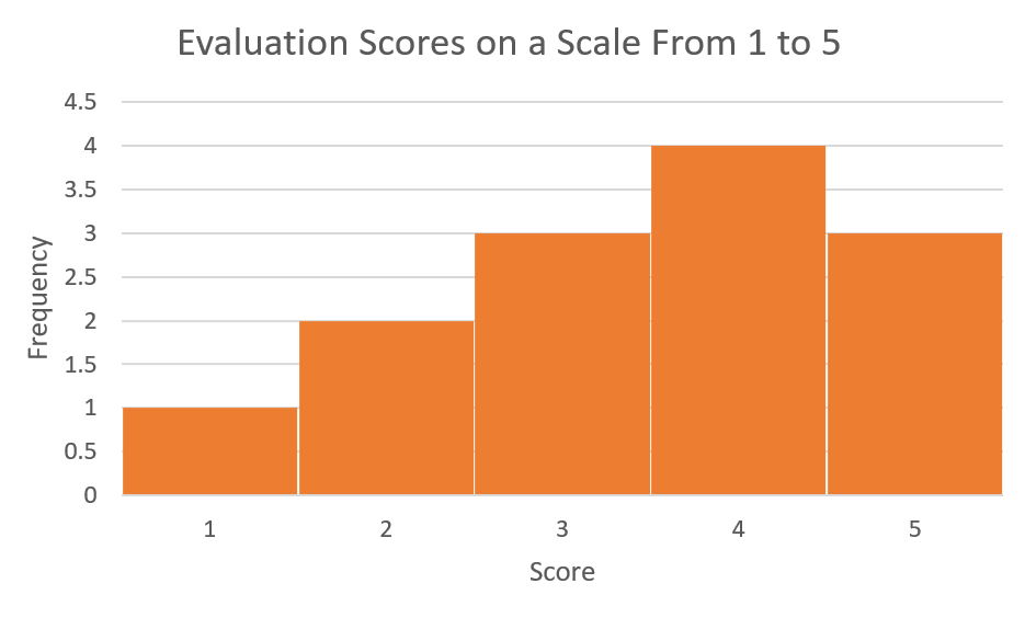
Referring to Figure 2, Instructor B received a mix of scores. Figure 2 represents a skewed distribution where one tail of the distribution is stretched out more than the other.
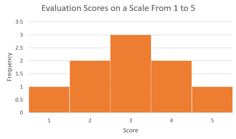
Referring to Figure 3, Instructor C also received a mix of scores. Figure 3 represents a symmetrical distribution. Data values occur most often in the centre of the distribution and spread out equally on either side.
The histogram in Figure 3 is symmetric but because it represents a very small sample size it appears to be a series of rectangles stacked side by side. As the sample size increases a symmetrical distribution will become less boxy as illustrated in Figures 4 & 5.


Eventually if we consider the entire population the distribution will approach what is called the normal distribution as in Figure 6. This distribution is also called the bell curve.
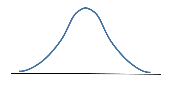
The normal distribution models many aspects of real life, including height, blood pressure and IQ scores.
Normal Distribution
The normal distribution is also called the bell curve.
In a normal distribution the data values are symmetrical around a vertical line drawn through its centre which is also where the mean is located. Half of the data values lie on either side of the mean.
In a normal distribution the mean, median and mode will all be equal.
Normal Distribution and Standard Deviation
The normal distribution will have symmetry in relation to the mean but it could be flat or high, depending on the standard deviation. In Figure 7 the means are identical but the distribution in A has a smaller standard deviation.

The standard deviation plays an important role in the normal distribution, as described by the 68-95-99.7 Rule.
68-95-99.7 Rule
According to the 68-95-99.7 Rule:
- Approximately 68% (68.26%) of the data items lie within one standard deviation of the mean.
- Approximately 95% (95.44%) of the data items lie within two standard deviations of the mean.
- Approximately 99.7% of the data items lie within three standard deviations of the mean.
Figure 8 depicts the 68-95-99.7 Rule.
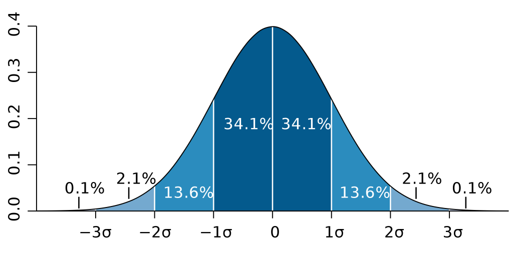
In simple language what does this rule tell us? Refer to Figure 8 and consider the percentage of data items that lie within one standard deviation (σ) of the mean. This is the region that lies between -1σ and 1σ. If 34.1% lie on either side of the mean, then 34.1% + 34.1% = 68.2% or approximately 68% . For a population with a normal distribution, just over two-thirds of the data (68%) will lie within one standard deviation of the mean.
Consider the percentage of data items that lie within two standard deviations of the mean. This is the region that lies between -2σ and 2σ. Between -2σ and 0, we find 13.6% + 34.1% or 47.7% of the data values. So between -2σ and 2σ we will have 47.7% + 47.7% = 95.4% or approximately 95% . For a population with a normal distribution, approximately 95% of the data values will lie within two standard deviations of the mean.
Consider the percentage of data items that lie within three standard deviations of the mean. This is the region that lies between -3σ and 3σ. Between -3σ and 0, we find 2.1% + 13.6% + 34.1% or 49.8% of the data values. So between -3σ and 3σ we will have 49.8% + 49.8% = 99.6%. (Note: The values in Figure 8 are all rounded to the nearest tenth. The number is actually closer to 49.86% x 2 = 99.72%). For a population with a normal distribution, approximately 99.7% of the data values will lie within three standard deviations of the mean. Another way of stating this, since 99.7% of the data will lie within three standard deviations of the mean, then only 0.3 % of the data will not lie within three standard deviations.
Using the 68-95-99.7 Rule
When working with a population that has a normal distribution the 68-95-99.7 Rule can be used to determine the percentage of the population that will be within one, two or three standard deviations of the mean.
EXAMPLE 1
A certain segment of the economy has a normally distributed salary, with a mean salary of $45,000 and a standard deviation of $4000.
a) Determine the salary that is one standard deviation above the mean.
b) Determine the salary that is three standard deviations below the mean.
c) Determine the salary range for the employees that lie within one standard deviation of the mean. What percent of the employees lie in this salary range?
d) Determine the salary range for the employees that lie within two standard deviations of the mean. What percent of the employees lie in this salary range?
e) What percent of the employees earn a salary less than $33,000?
Solution
a) $45,000 + $4000 = $49,000
b) $45,000 – (3 x $4000) = $33,000
c) $45,000 ± $4000 = $41,000 to $49,000. According to the 68-95-99.7 Rule, sixty-eight percent of the employees for this segment of the economy lie within this salary range.
d) $45,000 ± (2 x $4000) = $37,000 to $53,000. According to the 68-95-99.7 Rule, ninety-five percent of the employees for this segment of the economy lie within this salary range.
e) A salary of $33,000 is 3 standard deviations below the mean. According to the 68-95-99.7 Rule, 100% – 99.7% or 0.3% of the employees lie above or below three standard deviations from the mean. Dividing 0.3 in half, we determine that 0.15% of the employees earn a salary less than $33,000.
TRY IT 1
Birth weights for newborns follow a normal distribution with a mean birth weight of 3.4 kg and a standard deviation of 0.55 kg. (Source O’Cathain et al)
a) Determine the birth weight that is two standard deviations above the mean.
b) Determine the birth weight that is one standard deviation below the mean.
c) Determine the weight range for newborns that lie within two standard deviations of the mean. What percent of the newborns lie in this weight range?
d) Determine the weight range for newborns that lie within three standard deviations of the mean. What percent of the newborns lie in this weight range?
e) What percent of newborns have a mean birth weight greater than 4.5 kg?
O’Cathain A., Walters S.J., Nicholl J.P., Thomas K.J., & Kirkham M. Use of evidence based leaflets to promote informed choice in maternity care: randomised controlled trial in everyday practice. British Medical Journal 2002; 324: 643-646
Show answer
a) 4.5 kg
b) 2.85 kg
c) 2.3 kg to 4.5 kg; 95% of newborns will have birth weights in this range
d) 1.75 kg to 5.05 kg which is 99.7% of the newborns
e) 0.15% of newborns
When we know the total number of data items in the population we are able to extend beyond stating percentages. This is illustrated in the Example 2.
EXAMPLE 2
A final exam was administered to 150 students enrolled in a first year calculus course. The mean score on the exam was 67% with a standard deviation of 8.
a) Determine the number of students who received a score of 67% or greater.
b) Determine the number of students who received a score within one standard deviation of the mean. What was the range in scores for these students?
c) Determine the number of students who received a score ranging between 51% to 83%.
d) What possible scores did the top 0.15% of the students receive? How many students were in this group?
Solution
a) Since 67% was the mean or average score, half of the students 0.5 x 150 = 75 students received a score of 67% or greater.
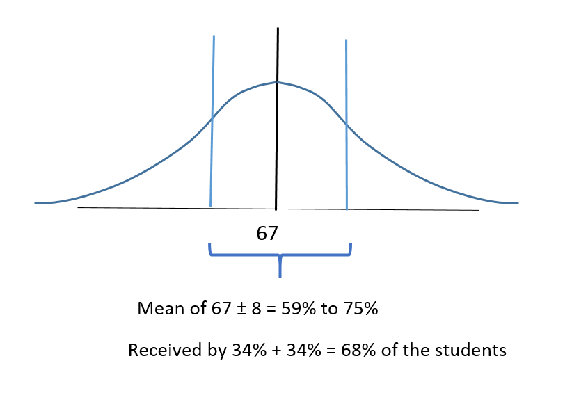
b) According to the Rule, one standard deviation on either side of the mean represents 34% + 34% = 68% of the students so
0.68 x 150 students = 102 students scored within one standard deviation of the mean.
We know that the mean score was 67% and one standard deviation of 8 on either side:
67 – 8 = 59% and 67 + 8 = 75% therefore the 102 students within one standard deviation scored from 59% to 75% on the exam.
c) If we consider the mean of 67% and two standard deviations on either side:
67 – (2×8) = 51% and 67 + (2×8) = 83% This indicates that students who scored from 51% to 83% were two standard deviations on either side of the mean.
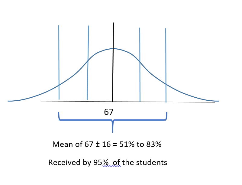
According to the Rule, two standard deviations on either side represents 95% of the students therefore 0.95 x 150 = 142.5 or between 142 to 143 students scored between 51% and 83% on the exam.
d) According to the Rule, 99.7% of the exam scores lie within 3 standard deviations of the mean, so 0.15% of the students scored higher than 3 standard deviations above the mean score. The mean score was 67% so:
67% + 3 standard deviations of 8 = 67% + (3 x 8) = 67% + 24% = 91%
Therefore the top 0.15% of the students received exam scores greater than 91%
The number of students receiving this score would be 0.15% x 150 students = 0.0015 x 150 = 0.225 students. This indicates that at most one student received a score greater than 91%.
TRY IT 2
A local run club hosted a recreational race. There were 148 entrants in the men’s category and the mean time (rounded to the nearest minute) was 120 minutes with a standard deviation of 15 minutes.
a) Determine the number of runners who had times of 2 hours (120 minutes) or less.
b) Determine the number of runners who clocked a time within one standard deviation of the mean. What were the possible times for these runners?
c) Determine the number of runners who recorded a time between 90 and 150 minutes. (Hint: Consider that one standard deviation is 15 minutes)
d) What possible times did the slowest 2.5% of the runners record? How many runners were in this group?
Show answer
a) 0.5 x 148 = 74 runners
b) 0.68 x 148 = 100.6 runners (100 to 101) runners; 120 min. ± 15 min. = 105 to 135 min.
c) mean ± 2 std. deviations = 120 ± 30 min. = 90 to 150 minutes so this is 95% of the runners. 0.95 x 148 = 140.6 (140 to 141 runners)
d) 5% of the runners had times either two standard deviations above or below the mean so 2.5 % had times above the mean (the slowest times). 120 min + (2 x 15min) = 150 min. or greater
For 2.5% of 148 = 3.7 so 3 to 4 runners.
When working with a population that is normally distributed, it can be helpful to sketch the normal curve and calculate values that are one, two and three standard deviations on either side of the mean.
EXAMPLE 3
The average salary for a certain occupation in the trades is determined to be $46,000 (rounded to the nearest thousand) and the standard deviation is $3000. The salaries are normally distributed as indicated in the figure:
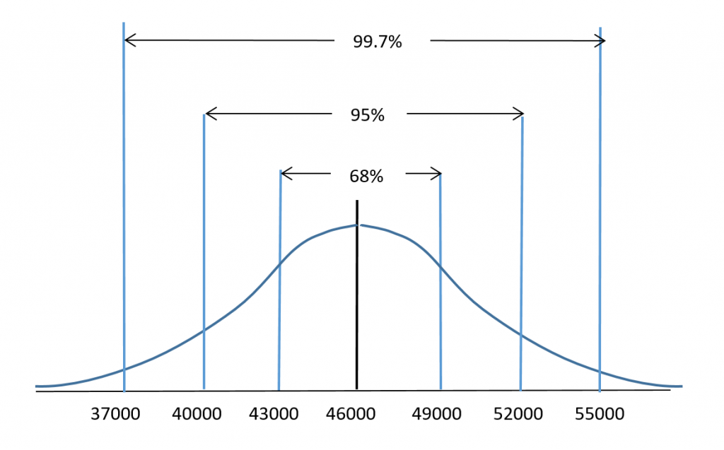
Use the 68-95-99.7 rule to determine the percentage of workers in this trade who earn:
a) less than $46,000
b) between $43,000 and $49,000
c) between $37,000 and $55,000
d) less than $55,000
e) between $40,000 and $49,000
Solution:
Note that there is more than one approach for these.
a) Since $46,000 is the mean, 50% of the workers will earn less than $46,000.
b) $43000 is one standard deviation less than the mean and $49,000 is one standard deviation more than the mean. Using the Rule, 68% of the workers will earn between $43000 and $46000.
c) $37000 is three standard deviations less than the mean and $55,000 is three standard deviations more than the mean. Using the Rule, 99.7% of the workers will earn between $37000 and $55000.
d) From the Rule, 99.7% of the data values lie between 3 standard deviations or $37000 to $55000. The remaining 100% – 99.7% = 0.3% of the data values lie equally at either end of the distribution. This means that 0.3% /2 or 0.15% of the data values are greater than $55000 and 0.15% are less than $37,000. So 99.7% + 0.15% = 99.85% of the workers will earn less than $55000.
e) One approach is to work the two halves of the distribution separately and then add the results.
Start with the data values that lie between $40000 and the mean of $46000. The salary of $40000 is is two standard deviations below the mean. If 95% of the values are ± 2 standard deviations from the mean then half this amount 95%/2 = 47.5% of the values are between $40000 and $46000.
Now consider $49000 which is one standard deviation greater than the mean. If 68% of the values are ± 1 standard deviation from the mean then half this amount 68%/2 = 34% of the values are between $46000 and $49000.
Now add the two percentages 47.5% + 34% = 81.5%. Therefore 81.5% of the workers earn between $40000 and $49000.
TRY IT 3
A physics exam worth 90 points was administered to all first year students. The mean score was 53 points with a standard deviation of 10 points. The scores were normally distributed as indicated in the figure:
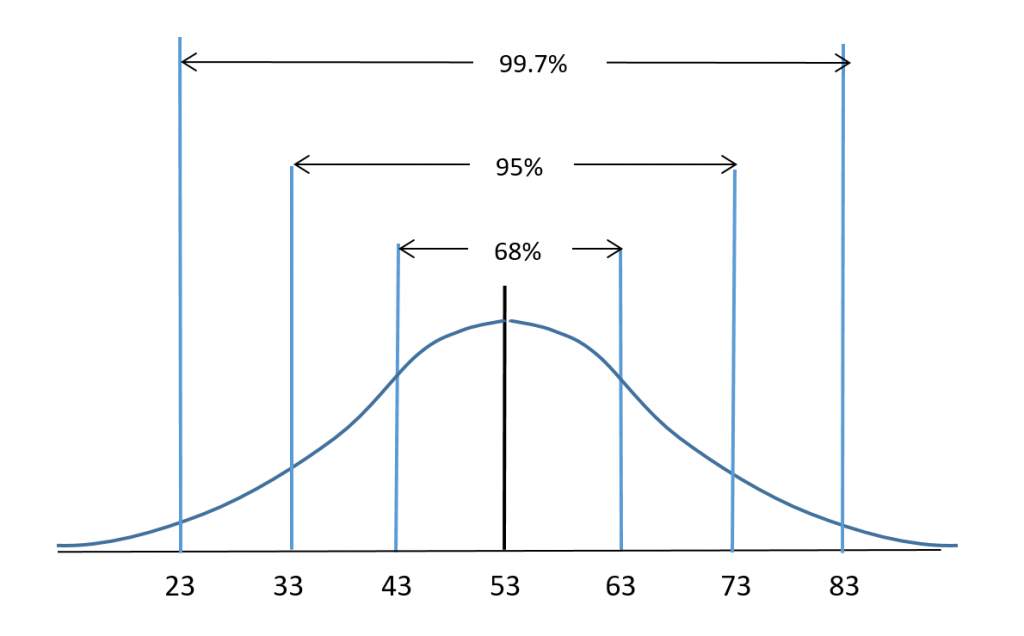
Use the 68-95-99.7 rule to determine the percentage of students who scored:
a) less than 63 points
b) between 33 and 53 points
c) more than 73 points
d) between 43 and 83 points
e) less than 43 points
Show answer
a) 50% + 34% = 84%
b) 95%/2 = 47.5%
c) 100% – 95% = 5% split evenly for scores less than 33 and greater than 73 so 5%/2 = 2.5% scored more than 73.
d) 34% + 99.7%/2 = 83.85%
e) 50% – 68%/2 = 16%
Key Concepts
- The normal distribution is also called the bell curve. The data values have a symmetrical distribution around a vertical line drawn through the mean.
- When working with a population that has a normal distribution the 68-95-99.7 Rule can be used to determine the proportion of the population that will lie within one, two or three standard deviations of the mean.
- 68% of the data values will lie within 1 standard deviation of the mean
- 95% of the data values will lie within 2 standard deviations of the mean
- 99.7% of the data values will lie within 3 standard deviations of the mean
Glossary
Normal Distribution
is when the data values lie in a symmetric fashion around the mean. Half of the data values lie on either side of the mean.
Skewed Distribution
is when more of the data values lie at one end of the distribution as compared to the other end.
8.3 Exercise Set
- A population’s average weight is normally distributed.
- What percent of the population will have an average weight that lies within one standard deviation of the mean?
- What percent of the population will have an average weight that lies within three standard deviations of the mean?
- What percent of the population will have an average weight that lies beyond three standard deviations of the mean?
- A certain segment of the economy has a normally distributed salary, with a mean salary of $72,000 and a standard deviation of $8000.
- Determine the salary that is one standard deviation below the mean.
- Determine the salary that is two standard deviations above the mean.
- Determine the salary range for the employees that lie within one standard deviation of the mean. What percent of the employees lie in this salary range?
- Determine the salary range for the employees that lie within three standard deviations of the mean. What percent of the employees lie in this salary range?
- What percent of the employees earn a salary more than $72,000?
- The average salary for a certain professional occupation is determined to be $76,000 (rounded to the nearest thousand) and the standard deviation is $6000. The salaries are normally distributed as indicated in the figure:
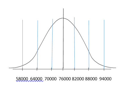 Use the 68-95-99.7 rule to determine the percentage of professionals in this occupation who earn:
- more than $76,000
- between $70,000 and $82,000
- between $64,000 and $88,000
- less than $58,000
- between $76,000 and $88,000
- between $58,000 and $76,000
- more than $82,000
- A survey of 100 people indicated that the average daily time they spend watching television is 2.5 hours with a standard deviation of 0.75 hours (45 minutes).
- Determine the amount of TV time that is one standard deviation above or below the average.
- Determine the amount of TV time that is two standard deviations above or below the average.
- Determine the amount of TV time that is more than three standard deviations above the average.
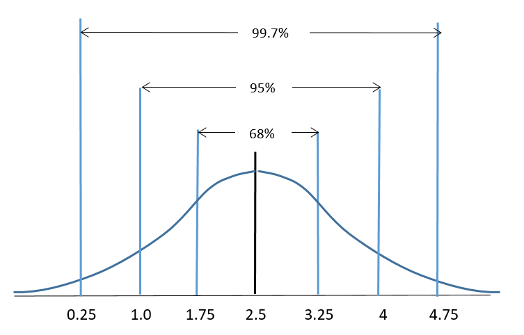
- A survey of 200 people indicated that the average daily time they spend watching television is 2.5 hours with a standard deviation of 0.75 hours (45 minutes).
- Sketch a normal distribution and label the TV times (in hours) that represent the mean and the standard deviations from the mean. (Hint: Refer to your answers for question #4)
- What percent of those surveyed will watch TV for more than 4.75 hours/day? How many people out of the group watch TV for more than 4.75 hours/day?
- What percent of those surveyed will watch TV for less than 2.5 hours/day? How many people out of the group watch TV for less than 2.5 hours/day?
- What percent of those surveyed will watch TV for less than 1.75 hours/day? How many people out of the group watch TV for less than 1.75 hours/day?
- What percent of those surveyed will watch TV between 1.75 hours/day and 4 hours/day? How many people out of the group watch TV for 1.75 to 4 hours/day?
- What percent of those surveyed will watch TV between 0.25 hours/day and 3.25 hours/day? How many people out of the group watch TV for 0.25 to 3.25 hours/day?
- A local run club hosted a recreational race. There were 230 entrants in the women’s category and the mean time (rounded to the nearest minute) was 135 minutes with a standard deviation of 15 minutes.
- Determine the number of runners who had times of 135 minutes or more.
- Determine the number of runners who recorded a time greater than one standard deviation from the mean. What were the possible times for these runners?
- Determine the number of runners who recorded a time between 105 and 135 minutes. (Hint: Consider that one standard deviation is 15 minutes)
- What possible times did the fastest 0.15% of the runners record? How many runners were in this group
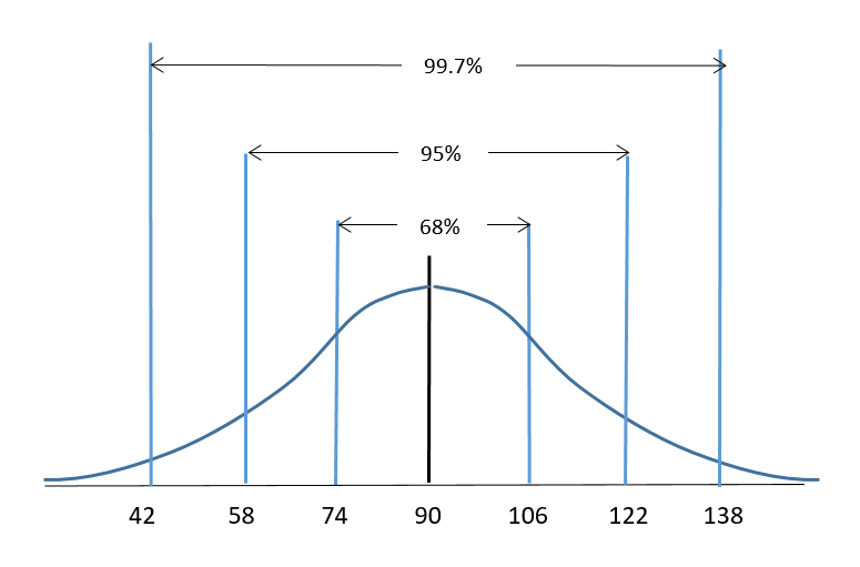
- A biology exam worth 140 points was administered to all first year students. The mean score was 90 points with a standard deviation of 16 points. The scores were normally distributed. Sketch the normal curve and calculate and label the scores that are one, two and three standard deviations on either side of the mean.
- A biology exam worth 140 points was administered to all first year students. The mean score was 90 points with a standard deviation of 16 points. The scores were normally distributed. Refer to the sketch in question#7 and use the 68-95-99.7 rule to determine the percentage of students who scored:
- more than 106 points
- between 74 and 106 points
- less than 58 points
- between 74 and 122 points
- more than 122 points
- between 42 and 74 points
- Your teacher informs you that your exam score was one standard deviation less than the mean. What percentile would this be?
- Your teacher informs you that your exam score was exactly three standard deviations greater than the mean. What percentile would this be?
Answers
-
- 68%
- 99.7%
- 100% – 99.7% = 0.3%
-
- $64,000
- $88,000
- $64,000-$80,000; 68%
- $48,00-$96,000; 99.7%
- 50%
-
- 50%
- 68%
- 95%
- (100% – 99.7%)/2 = 0.15%
- 95%/2 = 47.5% f) 99.7%/2 = 49.85% g) 100% – (34% + 50%) = 16%
-
- 1.75 to 3.25 hours
- 1 to 4 hours
- more than 4.75 hours
-
- (100% – 99.7%)/2 = 0.15%; 30 people
- 50%; 100 people
- 50% – (68%/2) = 16%; 32 people
- 34% + (95% ÷ 2) = 81.5%; 163 people
- (99.7% ÷ 2) + 34% = 83.85%; ≈168 people
-
- 50% so 115 runners
- 36.6 so between 36 and 37
- 109.25 so between 109 and 110
- less than 90 minutes; at most one runner
-
- 16%
- 68%
- 2.5%
- 81.5%
- 2.5%
- 15.85%
- 50% – 68%/2 = 16% of the data values lie below this so this is the 16th percentile
- 99th percentile
