Earth-system interactions are so complex that it is next to impossible to follow all of the connections and implications without help. So, scientists use Earth-system computer models to assist. Earth-system models incorporate knowledge of the many components of the Earth system in a way that makes it possible to test how important any one change is.

Earth-system models vary in how many aspects of the Earth system they include, and how detailed their representations of those aspects are. Models are designed to answer particular kinds of questions so their performance can be optimized; a study that is concerned only with large-scale global changes might not require a model with a highly detailed representation of Earth’s coastlines. It takes more time to run a complicated model, so this saves on computing resources.

When computer models are discussed, we acknowledge that there is a difference between measurements of the real world, and the output from the model. Modelers are careful to refer to measurements of the real word as data, and output from the model as results. This also helps to avoid confusion when comparing models to real-world measurements to gauge how realistic the model output is.

What Are Computer Models, Exactly?

Computer models describe natural phenomena using mathematical equations. On the most basic level, computer models take some quantity—whether heat, water, or the concentration of a pollutant—and calculate how it moves through a system. Sometimes they look only at how that quantity changes through time. A computer model of the water volume in a bathtub could be limited to looking at how rapidly water flows in through the tap, and how rapidly it flows out through the drain. But sometimes models look at how a quantity changes in space as well as through time.

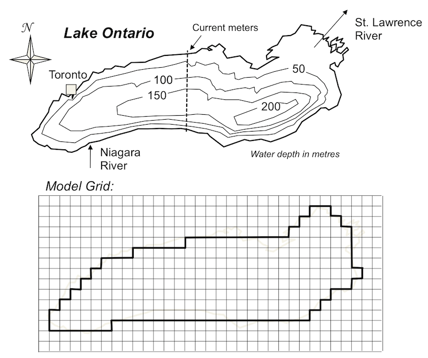
A study of wind-driven currents in a lake must include information about the shape and depth of the lake to capture how friction at the lake bottom and along the sides affects water flow (Figure 16.28). Data about the lake shape and depth (Figure 16.28, top) is translated to a model grid (Figure 16.28, bottom). Calculations are done to see how wind and friction control how water moves into and out of each cell in the grid.

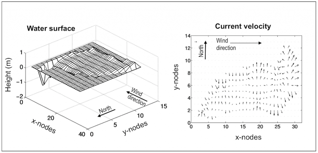
The model produces information about wave height (Figure 16.29, left) and shows the direction and speed of water flow across the lake using arrows of different sizes (Figure 16.29, right). If scientists are interested in how a pollutant would move around the lake, they can include the location where the pollutant is added, and how rapidly it is added, and track how it moves.

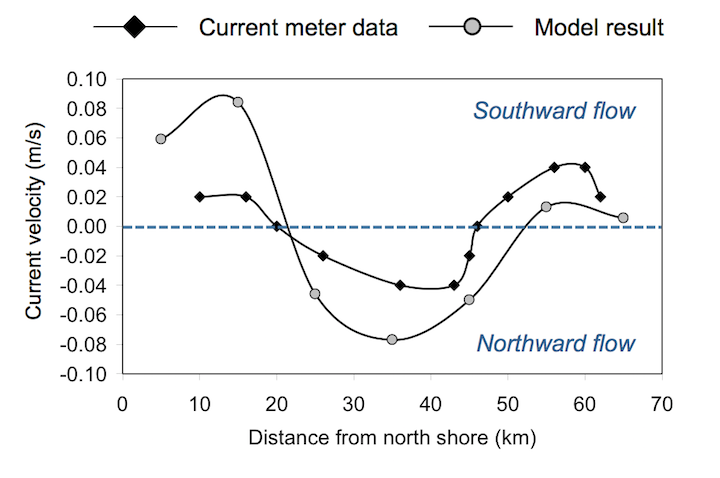
If the model is to be used to track the movement of a pollutant through the lake, it is important to know that it has done a good job of calculating the current velocity. In this case, data from current meters in the lake can be compared to the current velocities that the model calculates (Figure 16.30). The model captures the fact that flow is northward near the margins of the lake, and southward in the middle, but the model current velocities are not exactly the same. This means that the model would do a good job of predicting where the pollution went, but not as good a job at predicting how fast it got there.

The model in this case had a relatively course representation of the lake geography, so a first step would be to make the grid cells smaller to do a better job of simulating the shape of the lake, then look at the flow in finer detail. Another step would be to represent the lake water using a vertical stack of several grid cells to better capture the extent to which bottom friction and wind force affect the lake water at different depths, and to do a better job of representing the water depth.

An Example of Using a Computer Model to Study Past Earth-System Change

The Paleocene-Eocene Thermal Maximum (PETM) was a sudden global warming event that happened approximately 56 million years ago. There was interest in studying this event because its suddenness was thought to be a good analogy for the rapid changes happening in the Earth system today. Cores from ocean-floor rocks show that the oceans became so acidified during the PETM that calcium carbonate sediments dissolved over vast areas of the ocean floor, vanishing entirely from some regions. The same cores also showed a shift in the carbon-isotope composition of calcium carbonate sediments.

Both the acidification and the carbon-isotope shift indicated that a large amount of carbon was added to the Earth system to trigger the PETM. The problem was that there were a number of possible sources for the carbon, and thus a number of possible triggers for the event. Although scientists provided reasoned arguments for their favourite hypotheses, there was no way to know for sure which was the best answer.

To solve this problem, an Earth-system model was used that could test which scenario could best account for the pattern of dissolving calcium carbonate. It took into account the shape of ocean basins, ocean current circulation, and carbonate system chemistry in ocean water and in sediments. It also took into account changes in sediments once they were deposited.

The steps to using this model were the following:

1. A search was done to locate as many studies of ocean floor sampling sites as possible that had information about changes in the amount of calcium carbonate during the PETM.
2. The model was set up so that it did a good job of reproducing the distribution of calcium carbonate before the PETM happened. This was important to ensure that model scenarios began with a realistic set of conditions.
3. Each of the possible scenarios involved carbon coming from different sources in the Earth system, meaning that each scenario could be represented in the model by adding to the atmosphere different amounts of carbon with different carbon isotope compositions. The more carbon a scenario required, the more the calcium carbonate sediments would have dissolved in real life.
4. The model was run for each different amount of carbon. For each scenario, the pattern of calcium carbonate sediments that the model gave was compared to the actual distribution of calcium carbonate sediments known from the data collected in Step 1.

In the end, the model showed that some of the scenarios did not even come close to matching the observations, either dissolving way too much calcium carbonate, or far too little. The model showed that two scenarios did come close to reproducing the pattern of calcium carbonate, and that one did a better job of matching the observations than the other. When it came time to write a report about the experiments, the scientists learned that newly published measurements from another study supported the scenario that the model suggested was best. It would have been acceptable to write a paper describing the model results, and which scenario worked best. However, also being able to comment about new supporting data meant there was a better chance of convincing other scientists that the model results were meaningful.

Predicting the Future of the Earth System with Models

Using models to investigate the Earth system requires careful consideration of how to build the model and run experiments. But it also requires skillful use of real-life measurements to set up the model, and to interpret and evaluate its results. The PETM model study was an example of how a model can be used to test hypotheses about past behaviour of the Earth system. There were data from before, during, and after the event to help set up the model and gauge its effectiveness.

Using Earth-system models to predict the future is a different kind of modeling challenge, because we don’t already know what the right answer is. The situation being modeled hasn’t happened yet. Scientists who try to predict the future of the Earth system have to do things a bit differently in order to have some confidence in the reliability of their model outcomes:

• They must come up with reasonable forcing scenarios for the model. A model used to predict the future of Earth’s climate will need input about what atmospheric greenhouse gas levels will be. That will depend on what actions humans take. Scientists deal with this unknown variable by testing multiple scenarios for greenhouse gas levels, such as what would happen if fossils fuels continue to be used as they have been, or alternatively, what would happen if we completely stopped using fossil fuels tomorrow. The scenarios they choose span a range of possibilities, including extreme cases, to make sure they understand what the possible range of outcomes could be.
• Scientists use some of the data they have to set the model up so that it is a realistic representation of the Earth system at a particular time in history. They then test the model to see if it can reproduce a different set of data later in history. This is a way to see if the model can get the right answer for a time when we know the right answer. Finally, after determining that the model gives reasonable results for times when we know the right answer, it is run for future scenarios.
• To be confident about predictions of future Earth-system change, scientists may collaborate to run their scenarios on many different Earth-system models designed by many different research groups at many different institutions. These models are set up with slightly different mathematical representations of processes, or different levels of detail in geographic representations. The scientists who built the various models might disagree on what numbers to assign some of the variables, or even which parts of the Earth system are necessary to include. If all the models produce similar results for a particular scenario in spite of representing a wide range of ideas about how such models should work, scientists can be more confident in those results.
• Scientists report uncertainty with their model results. It is a common misconception that uncertainty means the same thing as in everyday language—that we just don’t know something, or can’t say for sure. But for models, uncertainty is a number that indicates the likelihood that a model result is within a certain range of values. It is determined using methods that are themselves the product of careful research. A meaningful discussion of uncertainty will concern a specific model or set of models, a specific variable, and include a specific range of values. It will also include information about how large the uncertainty is compared to the changes they are investigating. If these details are missing from the conversation, it’s a clue that “uncertainty” is being used in a common-language way rather than the way that modellers use it. Note that reporting uncertainty is not exclusive to models predicting the future, but it is particularly important for those models because of the great scrutiny Earth-system models receive when they are used to investigate future climate change.

References

Simons, T. J., & Schertzer, W. M. (1989) The circulation of Lake Ontario during the summer of 1982 and the winter of 1982/83. Burlington, ON: Environment Canada. http://publications.gc.ca/site/eng/9.854046/publication.html

Slingerland, R., & Kump, L. (2011). Mathematical Modeling of Earth’s Dynamical Systems: A Primer. Princeton University Press.